Digital Image Forensics Using Sensor Noise

Digital Image Forensics Using Sensor Noise
Abstract—This tutorial explains how photo-response nonuniformity
(PRNU) of imaging sensors can be used for a
variety of important digital forensic tasks, such as device
identification, device linking, recovery of processing history,
and detection of digital forgeries. The PRNU is an intrinsic
property of all digital imaging sensors due to slight variations
among individual pixels in their ability to convert photons to
electrons. Consequently, every sensor casts a weak noise-like
pattern onto every image it takes. This pattern, which plays
the role of a sensor fingerprint, is essentially an unintentional
stochastic spread-spectrum watermark that survives
processing, such as lossy compression or filtering. This tutorial
explains how this fingerprint can be estimated from images
taken by the camera and later detected in a given image to
establish image origin and integrity. Various forensic tasks are
formulated as a two-channel hypothesis testing problem
approached using the generalized likelihood ratio test. The
performance of the introduced forensic methods is briefly
illustrated on examples to give the reader a sense of the
performance.
Index Terms—Photo-response non-uniformity, imaging
sensor, digital forensic, digital forgery, camera identification,
authentication, integrity verification.
I. INTRODUCTION
There exist two types of imaging sensors commonly
found in digital cameras, camcorders, and scanners⎯CCD
(Charge-Coupled Device) and CMOS (Complementary
Metal-Oxide Semiconductor). Both consist of a large
number of photo detectors also called pixels. Pixels are
made of silicon and capture light by converting photons
into electrons using the photoelectric effect. The
accumulated charge is transferred out of the sensor,
amplified, and then converted to a digital signal in an AD
converter and further processed before the data is stored in
an image format, such as JPEG.
The pixels are usually rectangular, several microns
across. The amount of electrons generated by the light in a
pixel depends on the physical dimensions of the pixel
photosensitive area and on the homogeneity of silicon. The
pixels' physical dimensions slightly vary due to
imperfections in the manufacturing process. Also, the
inhomogeneity naturally present in silicon contributes to
variations in quantum efficiency among pixels (the ability
to convert photons to electrons). The differences among
pixels can be captured with a matrix K of the same
dimensions as the sensor. When the imaging sensor is
illuminated with ideally uniform light intensity Y, in the
absence of other noise sources, the sensor would register a
noise-like signal Y+YK instead. The term YK is usually
referred to as the pixel-to-pixel non-uniformity or PRNU.
Jessica Fridrich
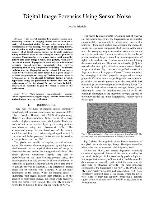
The matrix K is responsible for a major part of what we
call the camera fingerprint. The fingerprint can be estimated
experimentally, for example by taking many images of a
uniformly illuminated surface and averaging the images to
isolate the systematic component of all images. At the same
time, the averaging suppresses random noise components,
such as the shot noise (random variations in the number of
photons reaching the pixel caused by quantum properties of
light) or the readout noise (random noise introduced during
the sensor readout), etc. The reader is referred to [1,2] for a
more detailed description of various noise sources affecting
image acquisition. Fig. 1 shows a magnified portion of a
fingerprint from a 4 megapixel Canon G2 camera obtained
by averaging 120 8-bit grayscale images with average
grayscale 128 across each image. Bright dots correspond to
pixels that consistently generate more electrons, while dark
dots mark pixels whose response is consistently lower. The
variance in pixel values across the averaged image (before
adjusting its range for visualization) was 0.5 or 51 dB.
Although the strength of the fingerprint strongly depends on
the camera model, the sensor fingerprint is typically quite a
weak signal.
Fig. 1: Magnified portion of the sensor fingerprint from Canon G2. The
dynamic range was scaled to the interval [0,255] for visualization.
Fig. 2 shows the magnitude of the Fourier transform of
one pixel row in the averaged image. The signal resembles
white noise with an attenuated high frequency band.
Besides the PRNU, the camera fingerprint essentially
contains all systematic defects of the sensor, including hot
and dead pixels (pixels that consistently produce high and
low output independently of illumination) and the so called
dark current (a noise-like pattern that the camera would
take with its objective covered). The most important
component of the fingerprint is the PRNU. The PRNU term
YK is only weakly present in dark areas where Y ≈ 0. Also,
completely saturated areas of an image, where the pixels
were filled to their full capacity, producing a constant
signal, do not carry any traces of PRNU or any other noise
for that matter.

We note that essentially all imaging sensors (CCD,
CMOS, JFET, or CMOS-Foveon X3) are built from
semiconductors and their manufacturing techniques are
similar. Therefore, these sensors will likely exhibit
fingerprints with similar properties.
|F|
80
70
60
50
40
30
20
10
0
0 200 400 600
Frequency
800 1000 1200
Fig. 2: Magnitude of Fourier transform of one row of the sensor
fingerprint.
Even though the PRNU term is stochastic in nature, it is a
relatively stable component of the sensor over its life span.
The factor K is thus a very useful forensic quantity
responsible for a unique sensor fingerprint with the
following important properties:
1. Dimensionality. The fingerprint is stochastic in nature
and has a large information content, which makes it unique
to each sensor.
2. Universality. All imaging sensors exhibit PRNU.
3. Generality. The fingerprint is present in every picture
independently of the camera optics, camera settings, or
scene content, with the exception of completely dark
images.
4. Stability. It is stable in time and under wide range of
environmental conditions (temperature, humidity).
5. Robustness. It survives lossy compression, filtering,
gamma correction, and many other typical processing.
The fingerprint can be used for many forensic tasks:
• By testing the presence of a specific fingerprint in the
image, one can achieve reliable device identification
(e.g., prove that a certain camera took a given image)
or prove that two images were taken by the same
device (device linking). The presence of camera
fingerprint in an image is also indicative of the fact that
the image under investigation is natural and not a
computer rendering.
• By establishing the absence of the fingerprint in
individual image regions, it is possible to discover
maliciously replaced parts of the image. This task
pertains to integrity verification.
• By detecting the strength or form of the fingerprint, it is
possible to reconstruct some of the processing history.
For example, one can use the fingerprint as a template
to estimate geometrical processing, such as scaling,
cropping, or rotation. Non-geometrical operations are
also going to influence the strength of the fingerprint in
the image and thus can be potentially detected.
• The spectral and spatial characteristics of the
fingerprint can be used to identify the camera model or
distinguish between a scan and a digital camera image
(the scan will exhibit spatial anisotropy).
In this tutorial, we will explain the methods for
estimating the fingerprint and its detection in images. The
material is based on statistical signal estimation and
detection theory.
The paper is organized as follows. In Section II, we
describe a simplified sensor output model and use it to
derive a maximum likelihood estimator for the fingerprint.
At the same time, we point out the need to preprocess the
estimated signal to remove certain systematic patterns that
might increase false alarms in device identification and
missed detections when using the fingerprint for image
integrity verification. Starting again with the sensor model
in Section III, the task of detecting the PRNU is formulated
as a two-channel problem and approached using the
generalized likelihood ratio test in Neyman-Pearson setting.
First, we derive the detector for device identification and
then adapt it for device linking and fingerprint matching.
Section IV shows how the fingerprint can be used for
integrity verification by detecting the fingerprint in
individual image blocks. The reliability of camera
identification and forgery detection using sensor fingerprint
is illustrated on real imagery in Section V. Finally, the
paper is summarized in Section VI.
Everywhere in this paper, boldface font will denote
vectors (or matrices) of length specified in the text, e.g., X
and Y are vectors of length n and X[i] denotes the ith
component of X. Sometimes, we will index the pixels in an
image using a two-dimensional index formed by the row
and column index. Unless mentioned otherwise, all
operations among vectors or matrices, such as product,
ratio, raising to a power, etc., are elementwise. The dot
n
product of vectors is denoted as XY = ∑ X[] i Y[]
i
i=
1
with || X||= XX being the L2 norm of X. Denoting the
sample mean with a bar, the normalized correlation is
( X−X) ( Y−Y) corr(
XY , ) =
.
|| X−X|| ⋅|| Y−Y|| II. SENSOR FINGERPRINT ESTIMATION
The PRNU is injected into the image during acquisition
before the signal is quantized or processed in any other
manner. In order to derive an estimator of the fingerprint,
we need to formulate a model of the sensor output.
A. Sensor Output Model
Even though the process of acquiring a digital image is
quite complex and varies greatly across different camera
models, some basic elements are common to most cameras.
The light cast by the camera optics is projected onto the
pixel grid of the imaging sensor. The charge generated

through interaction of photons with silicon is amplified and
quantized. Then, the signal from each color channel is
adjusted for gain (scaled) to achieve proper white balance.
Because most sensors cannot register color, the pixels are
typically equipped with a color filter that lets only light of
one specific color (red, green, or blue) enter the pixel. The
array of filters is called the color filter array (CFA). To
obtain a color image, the signal is interpolated or
demosaicked. Finally, the colors are further adjusted to
correctly display on a computer monitor through color
correction and gamma correction. Cameras may also
employ filtering, such as denoising or sharpening. At the
very end of this processing chain, the image is stored in the
JPEG or some other format, which may involve
quantization.
Let us denote by I[i] the quantized signal registered at
pixel i, i = 1, …, m×n, before demosaicking. Here, m×n are
image dimensions. Let Y[i] be the incident light intensity at
pixel i. We drop the pixel indices for better readability and
use the following vector form of the sensor output model
γ
γ
I= g ⋅ ( 1+ K) Y+ Ω + Q . (1)
[ ]
We remind the reader that all operations in (1) (and
everywhere else in this tutorial) are element-wise. In (1), g
is the gain factor (different for each color channel) and γ is
the gamma correction factor (typically, γ ≈ 0.45). The
matrix K is a zero-mean noise-like signal responsible for
the PRNU (the sensor fingerprint). Denoted by Ω is a
combination of the other noise sources, such as the dark
current, shot noise, and read-out noise [2]; Q is the
combined distortion due to quantization and/or JPEG
compression.
In parts of the image that are not dark, the dominant term
in the square bracket in (1) is the scene light intensity Y. By
factoring it out and keeping the first two terms in the Taylor
expansion of (1 + x) γ = 1 + γ x + O(x 2 ) at x = 0, we obtain
γ
γ
[ ]
I= ( gY)
⋅ 1+ K+ Ω / Y + Q
γ
(0) (0)
( gY)
⋅ ( 1+ γK+ γΩ/
Y) + Q= I + I K+ Θ.
γ
In (2), we denoted (0)
I = ( gY
) the ideal sensor output in
(0)
the absence of any noise or imperfections. Note that I K
(0)
is the PRNU term and Θ = γ I Ω / Y+ Q is the modeling
noise. In the last expression in (2), the scalar factor γ was
absorbed into the PRNU factor K to simplify the notation.
B. Sensor Fingerprint Estimation
In this section, the above sensor output model is used to
derive an estimator of the PRNU factor K. A good
introductory text on signal estimation and detection is [3,4].
(0)
The SNR between the signal of interest I K and
observed data I can be improved by suppressing the
(0)
noiseless image I by subtracting from both sides of (2) a
(0)
denoised version of I, Iˆ = F()
I , obtained using a
denoising filter F (Appendix A describes the filter used in
experiments in this tutorial):
(2)
ˆ(0) (0) ˆ (0) (0)
( )
W = I− I = IK+ I −I + I − I K+ Θ
(3)
= IK + Ξ .
It is easier to estimate the PRNU term from W than from
I because the filter suppresses the image content. We
denoted by Ξ the sum of Θ and two additional terms
introduced by the denoising filter.
Let us assume that we have a database of d ≥ 1 images,
I1, …, Id, obtained by the camera. For each pixel i, the
sequence 1 , …, is modeled as white Gaussian
noise (WGN) with variance σ
[] i Ξ d[] i Ξ
2
. The noise term is
technically not independent of the PRNU signal IK due to
(0)
the term ( I − I) K . However, because the energy of this
term is small compared to IK, the assumption that Ξ is
independent of IK is reasonable.
From (3), we can write for each k = 1, …, d
Wk Ξk
ˆ(0) ˆ(0)
= K+ , Wk = Ik − Ik , Ik
= F(
I k)
. (4)
Ik Ik
Under our assumption about the noise term, the loglikelihood
of observing W / I given K is
k k
d
∑
k= 1
2
k
2
d
2
( Wk / Ik − K)
∑ 2 2
k= 1 σ /( Ik
)
d
L( K) =− log(2 πσ /( I ) ) −
. (5)
2 2
By taking partial derivatives of (5) with respect to
individual elements of K and solving for K, we obtain the
maximum likelihood estimate ˆK
∂L(
) W / I − K
= ∑ = 0
∂ K
⇒ Kˆ
=
K I
d
k k
2 2
k= 1 σ /( k )
d
∑
k = 1
d
∑
k=
1
WI
k k
( I )
k
2
. (6)
The Cramer-Rao Lower Bound (CRLB) gives us the
bound on the variance of ˆK
d
2
2 ( k )
2
L(
) ∑ I
K k = 1
ˆ 1 σ
=− ⇒var K ≥ =
2 2 2
d
∂K σ
⎡∂L( K)
⎤
−E ⎢ 2 ⎥ ∑ Ik
k = 1
∂
( ) .
2
( )
⎣ ∂K
⎦
(7)
Because the sensor model (3) is linear, the CRLB tells us
that the maximum likelihood estimator is minimum
variance unbiased and its variance var( Kˆ
) ~ 1/d. From (7),
we see that the best images for estimation of K are those
2
with high luminance (but not saturated) and small σ
(which means smooth content). If the camera under
investigation is in our possession, out-of-focus images of
bright cloudy sky would be the best. In practice, good
estimates of the fingerprint may be obtained from 20–50
natural images depending on the camera. If sky images are
used instead of natural images, only approximately one half
of them would be enough to obtain an estimate of the same
accuracy.
The estimate ˆK
contains all components that are
systematically present in every image, including artifacts
introduced by color interpolation, JPEG compression, on-

sensor signal transfer [5], and sensor design. While the
PRNU is unique to the sensor, the other artifacts are shared
among cameras of the same model or sensor design.
Consequently, PRNU factors estimated from two different
cameras may be slightly correlated, which undesirably
increases the false identification rate. Fortunately, the
artifacts manifest themselves mainly as periodic signals in
row and column averages of ˆK and can be suppressed
simply by subtracting the averages from each row and
column. For a PRNU estimate ˆK with m rows and n
columns, the processing is described using the following
pseudo-code
n
r = 1/ n ˆ ∑ K[ i,
j]
i j=
1
for i = 1 to m { Kˆ '[ i, j] = Kˆ[
i, j] −rifor
j = 1, …, n}
m
c 1/ ˆ
j = m∑K '[ i,
j]
i=
1
for j = 1 to n { Kˆ ''[, i j] = Kˆ
'[, i j] −cjfor
i = 1, …, m}.
The difference Kˆ − Kˆ
'' is called the linear pattern (see Fig.
3) and it is a useful forensic entity by itself − it can be used
to classify a camera fingerprint to a camera model or brand.
As this topic is not detailed in this tutorial, the reader is
referred to [6] for more details.
Fig. 3: Detail of the linear pattern for Canon S40.
To avoid cluttering the text with too many symbols, in the
rest of this tutorial we will denote the processed fingerprint
Kˆ
'' with the same symbol Kˆ
.
We close this section with a note on color images. In this
case, the PRNU factor can be estimated for each color
channel separately, obtaining thus three fingerprints of the
same dimensions ˆ K R , Kˆ
G , and Kˆ B.
Since these three
fingerprints are highly correlated due to in-camera
processing, in all forensic methods explained in this
tutorial, before analyzing a color image under investigation
we convert it to grayscale and correspondingly combine the
three fingerprints into one fingerprint using the usual
conversion from RGB to grayscale
ˆ 0.3 ˆ 0.6 ˆ 0.1 ˆ
K = KR+ KG + KB. (8)
III. CAMERA IDENTIFICATION USING SENSOR
FINGERPRINT
This section introduces general methodology for
determining the origin of images or video using sensor
fingerprint. We start with what we consider the most
frequently occurring situation in practice, which is camera
identification from images. Here, the task is to determine if
an image under investigation was taken with a given
camera. This is achieved by testing whether the image noise
residual contains the camera fingerprint. Anticipating the
next two closely related forensic tasks, we formulate the
hypothesis testing problem for camera identification in a
setting that is general enough to essentially cover the
remaining tasks, which are device linking and fingerprint
matching. In device linking, two images are tested if they
came from the same camera (the camera itself may not be
available). The task of matching two estimated fingerprints
occurs in matching two video-clips because individual
video frames from each clip can be used as a sequence of
images from which an estimate of the camcorder fingerprint
can be obtained (here, again, the cameras/camcorders may
not be available to the analyst).
A. Device identification
We consider the scenario in which the image under
investigation has possibly undergone a geometrical
transformation, such as scaling or rotation. Let us assume
that before applying any geometrical transformation the
image was in grayscale represented with an m×n matrix
I[i, j], i = 1, …, m, j = 1, …, n. Let us denote as u the
(unknown) vector of parameters describing the geometrical
transformation, Tu. For example, u could be a scaling ratio
or a two-dimensional vector consisting of the scaling
parameter and unknown angle of rotation. In device
identification, we wish to determine whether or not the
transformed image
Z T () I
= u
was taken with a camera with a known fingerprint estimate
ˆK . We will assume that the geometrical transformation is
downgrading (such as downsampling) and thus it will be
−1
more advantageous to match the inverse transform Tu ( )
with the fingerprint rather than matching Z with a
downgraded version of .
Z
ˆK
We now formulate the detection problem in a slightly
more general form to cover all three forensic tasks
mentioned above within one framework. The fingerprint
detection is the following two-channel hypothesis testing
problem
where
H: 0 K1 ≠ K2
H: K = K (9)
1 1 2
W = I K + Ξ
T W T Z K + Ξ
1 1 1 1
−1 u ( 2) =
−1
u ( ) 2
2 .
(10)
In (10), all signals are observed with the exception of the
noise terms Ξ1 , 2 and the fingerprints K
Ξ 1 and K2.
Specifically, for the device identification problem, I1 ≡1,
W ˆ
1 = K estimated in the previous section, and Ξ1
is the
estimation error of the PRNU. K
is the PRNU from the
2

camera that took the image, W2 is the geometrically
transformed noise residual, and Ξ2
is a noise term. In
general, u is an unknown parameter. Note that since
1
T ( 2 and may have different dimensions, the
formulation (10) involves an unknown spatial shift between
both signals, s.
−
u W ) 1 W
Modeling the noise terms Ξ1 and 2 as white Gaussian
noise with known variances
Ξ
2 2
σ 1 , σ 2 , the generalized
likelihood ratio test for this two-channel problem was
derived in [7]. The test statistics is a sum of three terms:
two energy-like quantities and a cross-correlation term
E
E
t = max{ E ( us , ) + E ( us , ) + C(
us , )} , (11)
us ,
1 2
2 2
I1[ i, j]( W1[
i+ s1, j+ s2])
1( us , ) = ∑ 2 2 4 −2 −1
2
i, jσ1I1[,
i j] + σ1σ2 ( Tu ( Z )[ i+ s1, j+ s2])
( T ( Z)[ i+ s , j+ s ]) ( T ( W )[ i+ s , j+ s ])
−1 2 −1
u 1 2 u 2 1 2
2( us , ) = ∑ 2 −1
2 4 −2 2
i, j σ2( Tu( Z)[
i+ s1, j+ s2]) + σ2σ1 I1[
i, j]
C(
us , ) =
I [ i, j] W[ i, j]( T ( Z)[ i+ s , j+ s ])( T ( W )[ i+ s , j+ s ])
−1 −1
1 1 u 1 2 u 2 1 2
∑
2 2 2 −1
2
i, j σ2I1[, i j] + σ1(
Tu ( Z)[
i+ s1, j+ s2])
The complexity of evaluating these three expressions is
proportional to the square of the number of pixels, (m×n) 2 ,
which makes this detector unusable in practice. Thus, we
simplify this detector to a normalized cross-correlation
(NCC) that can be evaluated using fast Fourier transform.
Under H1, the maximum in (11) is mainly due to the
contribution of the cross-correlation term, C(u, s), that
exhibits a sharp peak for the proper values of the
geometrical transformation. Thus, a much faster suboptimal
detector is the NCC between X and Y maximized over all
shifts s1, s2, and u
m n
∑∑( X[ kl , ] − X)( Y[ k+ s1, l+ s2]
−Y)
k= 1 l=
1
NCC[ s1, s 2;
u]
=
,
X−X Y−Y (12)
which we view as an m×n matrix parameterized by u,
where
−1 −1
IW 1 1
Tu ( Z) Tu
( W2)
X= , Y =
.
2 2
2 2 2 −1 2 2 2 −1
σ I + σ T ( Z) σ I + σ T ( Z)
( u ) ( u )
2 1 1 2 1 1
(13)
A more stable detection statistics, whose meaning will
become apparent from error analysis later in this section,
that we strongly advocate to use for all camera
identification tasks, is the Peak to Correlation Energy
measure (PCE) defined as
2
2
NCC[ speak; u]
PCE( u)
=
, (14)
1
2
∑ NCC[; s u]
mn− | N | ss , ∉N
where for each fixed u, N is a small region surrounding the
peak value of NCC speak across all shifts s1, s2.
For device identification from a single image, the
fingerprint estimation noise Ξ1
is much weaker compared
to Ξ2
for the noise residual of the image under
2 2
investigation. Thus, σ1 = var( Ξ1) var( Ξ2)
= σ 2 and (12)
can be further simplified to a NCC between
ˆ
−1 −1
X= W1= K and Y= Tu ( Z) Tu
( W2)
.
Recall that I1 = 1 for device identification when its
fingerprint is known.
In practice, the maximum PCE value can be found by a
search on a grid obtained by discretizing the range of u.
Because the statistics is noise-like for incorrect values of u
and only exhibits a sharp peak in a small neighborhood of
the correct value of u, unfortunately, gradient methods do
not apply and we are left with a potentially expensive grid
search. The grid has to be sufficiently dense in order not to
miss the peak. As an example, we provide in this tutorial
additional details how one can carry out the search when
u = r is an unknown scaling ratio. The reader is advised to
consult [9] for more details.
PCE
250
200
150
100
50
0
0.4 0.5 0.6 0.7 0.8 0.9 1
scaling ratio
Fig. 4: Top: Detected peak in PCE(ri). Bottom: Visual representation of
the detected cropping and scaling parameters rpeak, speak. The gray frame
shows the original image size, while the black frame shows the image size
after cropping before resizing.
Assuming the image under investigation has dimensions
M×N, we search for the scaling parameter at discrete values
ri ≤ 1, i = 0, 1, …, R, from r0 = 1 (no scaling, just cropping)

down to rmin = max{M/m, N/n} < 1
1
ri= , i = 0,1, 2,... . (15)
1+ 0.005i
For a fixed scaling parameter ri, the cross-correlation (12)
does not have to be computed for all shifts s but only for
1
those that move the upsampled image Tr ( ) within the
i
dimensions of because only such shifts can be generated
by cropping. Given that the dimensions of the upsampled
image are M/r
− Z
ˆK
1
T ( )
− Z i × N/ri, we have the following range
ri
for the spatial shift s = (s1, s2)
0 ≤ s1 ≤ m – M/ri and 0 ≤ s2 ≤ n – N/ri. (16)
The peak of the two-dimensional NCC across all spatial
shifts s is evaluated for each ri using PCE(ri) (14). If
maxi PCE(ri) > τ, we decide H1 (camera and image are
matched). Moreover, the value of the scaling parameter at
which the PCE attains this maximum determines the scaling
ratio rpeak. The location of the peak speak in the normalized
cross-correlation determines the cropping parameters. Thus,
as a by-product of this algorithm, we can determine the
processing history of the image under investigation (see
Fig. 4). The fingerprint can thus play the role of a
synchronizing template similar to templates used in digital
watermarking. It can also be used for reverse-engineering
in-camera processing, such as digital zoom [9].
In any forensic application, it is important to keep the
false alarm rate low. For camera identification tasks, this
means that the probability, PFA, that a camera that did not
take the image is falsely identified must be below a certain
user-defined threshold (Neyman-Pearson setting). Thus, we
need to obtain a relationship between PFA and the threshold
on the PCE. Note that the threshold will depend on the size
of the search space, which is in turn determined by the
dimensions of the image under investigation.
Under hypothesis H0 for a fixed scaling ratio ri, the
values of the normalized cross-correlation NCC[s; ri] as a
function of s are well-modeled [9] as white Gaussian noise
() i
2
ζ ~ N(0,
σ i ) with variance that may depend on i.
Estimating the variance of the Gaussian model using the
2
sample variance ˆ σ i of NCC[s; ri] over s after excluding a
small central region N surrounding the peak
2 1
ˆ i [; i]
| |
r
2
σ = ∑ NCC s , (17)
mn−
N
ss , ∉N
we now calculate the probability pi that () i
ζ would attain
the peak value NCC[speak; rpeak] or larger by chance:
2 2
∞ x
x
− ∞
−
1 2
2
2 ˆ σ
1
i
2 ˆ σi
∫ ∫
pi= e dx= e
2πσˆ 2πσˆ
NCC[ speak
; rpeak ] i ˆ σ peak PCEpeak
i
⎛ ˆ σ
Q PCE
⎞
,
⎝ ⎠
peak
= ⎜ peak ⎟
ˆ σ i
dx
where Q(x) = 1 – Φ(x) with Φ(x) denoting the cumulative
distribution function of a standard normal variable N(0,1)
and PCEpeak = PCE(rpeak). As explained above, during the
search for the cropping vector s, we only need to search in
the range (16), which means that we are taking maximum
over ki = (m – M/ri + 1)×(n – N/ri + 1) samples of ζ (i) . Thus,
the probability that the maximum value of ζ (i) would not
i
exceed NCC[speak; rpeak] is ( 1−p.
After R steps in the
search, the probability of false alarm is
FA
i
)
k
∏(
i )
P = 1− 1−
p
R
i=
1
ki
. (18)
Since we can stop the search after the PCE reaches a
certain threshold, we have ri ≤ rpeak. Because 2 ˆ σ i is nondecreasing
in i, ˆ σ ˆ peak / σ i ≥ 1.
Because Q(x) is decreasing,
we have pi ≤ ( PCEpeak
)
Q = p.
Thus, because ki ≤ mn, we
obtain an upper bound on PFA
( p)
, (19)
max k
PFA ≤1− 1−
where k
max
R−1
= ∑ k is the maximal number of values of the
i=
0
i
parameters r and s over which the maximum of (11) could
be taken. Equation (19), together with p= Q( τ ) ,
determines the threshold for PCE, τ = τ (PFA, M, N, m, n).
This finishes the technical formulation and solution of
the camera identification algorithm from a single image if
the camera fingerprint is known. To provide the reader with
some sense of how reliable this algorithm is, we include in
Section V some experiments on real images. This algorithm
can be used with small modifications for the other two
forensic tasks formulated in the beginning of this section,
which are device linking and fingerprint matching.
B. Device linking
The detector derived in the previous section can be
readily used with only a few changes for device linking or
determining whether two images, I1 and Z, were taken by
the exact same camera [11]. Note that in this problem the
camera or its fingerprint is not necessarily available.
The device linking problem corresponds exactly to the
two-channel formulation (9) and (10) with the GLRT
detector (11). Its faster, suboptimal version is the PCE (14)
obtained from the maximum value of NCC[ s1, s2;
u]
over all
s1, s2; u (see (12) and (13)). In contrary to the camera
identification problem, now the power of both noise terms,
Ξ1 and 2 , is comparable and needs to be estimated from
observations. Fortunately, because the PRNU term IK is
much weaker than the modeling noise reasonable
estimates of the noise variances are simply
2
Ξ
Ξ,
2 2
ˆ σ1 = var( W ˆ 1), σ2
= var( W ).
Unlike in the camera identification problem, the search
for unknown scaling must now be enlarged to scalings
ri > 1 (upsampling) because the combined effect of

unknown cropping and scaling for both images prevents us
from easily identifying which image has been downscaled
with respect to the other one. The error analysis carries over
from Section III.A.
Due to space limitations we do not include experimental
verification of the device linking algorithm. Instead, the
reader is referred to [11].
C. Matching fingerprints
The last, fingerprint matching scenario corresponds to the
situation when we need to decide whether or not two
estimates of potentially two different fingerprints are
identical. This happens, for example, in video-clip linking
because the fingerprint can be estimated from all frames
forming the clip [12].
The detector derived in Section III.A applies to this
scenario, as well. It can be further simplified because for
matching fingerprints we have I1 = Z = 1 and (12) simply
becomes the normalized cross-correlation between X= Kˆ
1
1
and T ( ˆ
2)
.
−
Y = u K
For experimental verification of the fingerprint matching
algorithm for video clips, the reader is advised to consult
[12].
IV. FORGERY DETECTION USING CAMERA
FINGERPRINT
A different, but nevertheless important, use of the sensor
fingerprint is verification of image integrity. Certain types
of tampering can be identified by detecting the fingerprint
presence in smaller regions. The assumption is that if a
region was copied from another part of the image (or an
entirely different image), it will not have the correct
fingerprint on it. The reader should realize that some
malicious changes in the image may preserve the PRNU
and will not be detected using this approach. A good
example is changing the color of a stain to a blood stain.
The forgery detection algorithm tests for the presence of
the fingerprint in each B×B sliding block separately and
then fuses all local decisions. For simplicity, we will
assume that the image under investigation did not undergo
any geometrical processing. For each block, BBb,
the
detection problem is formulated as hypothesis testing
H0: b b
b
b)
= W Ξ
H1: W ˆ
b = IbKb + Ξ . (20)
Here, Wb is the block noise residual, Kˆ
b is the
corresponding block of the fingerprint, Ib
is the block
intensity, and Ξb
is the modeling noise assumed to be a
2
white Gaussian noise with an unknown variance σΞ
. The
likelihood ratio test is the normalized correlation
ρ ( ˆ
b = corr IK b b,
W . (21)
In forgery detection, we may desire to control both types
of error – failing to identify a tampered block as tampered
and falsely marking a region as tampered. To this end, we
will need to estimate the distribution of the test statistic
under both hypotheses.
The probability density under H0, p(x|H0), can be
estimated by correlating the known signal IKˆ
with noise
b b
residuals from other cameras. The distribution of ρb
under
H1, p(x|H1), is much harder to obtain because it is heavily
influenced by the block content. Dark blocks will have
lower value of correlation due to the multiplicative
character of the PRNU. The fingerprint may also be absent
from flat areas due to strong JPEG compression or
saturation. Finally, textured areas will have a lower value of
the correlation due to stronger modeling noise. This
problem can be resolved by building a predictor of the
correlation that will tell us what the value of the test
statistics ρb and its distribution would be if the block b was
not tampered and indeed came from the camera.
The predictor is a mapping that needs to be constructed
for each camera. The mapping assigns an estimate of the
correlation ρb to each triple (ib, fb, tb), where the individual
elements of the triple stand for a measure of intensity,
saturation, and texture in block b. The mapping can be
constructed for example using regression or machine
learning techniques by training them on a database of image
blocks coming from images taken by the camera. The block
size cannot be too small (because then the correlation ρb has
too large a variance). On the other hand, large blocks would
compromise the ability of the forgery detection algorithm to
localize. Blocks of 64×64 or 128×128 pixels work well for
most cameras.
A reasonable measure of intensity is the average intensity
in the block
1
ib= ∑I[]
i . (22)
| Bb
| i∈Bb
We take as a measure of flatness the relative number of
pixels, i, in the block whose sample intensity variance σI[i]
estimated from the local 3×3 neighborhood of i is below a
certain threshold
1
fb = { i∈ Bb
| σ I [] i < cI[]}
i , (23)
Bb
where c ≈ 0.03 (for Canon G2 camera). The best values of c
vary with the camera model.
A good texture measure should somehow evaluate the
amount of edges in the block. Among many available
options, we give the following example
1 1
tb
=
| | ∑ , (24)
B 1+ var ( F[
i])
b i∈Bb
where var5(F[i]) is the sample variance computed from a
local 5×5 neighborhood of pixel i for a high-pass filtered
version of the block, F[i], such as one obtained using an
edge map or a noise residual in a transform domain.
Since one can obtain potentially hundreds of blocks from
a single image, only a small number of images (e.g., ten)
are needed to train (construct) the predictor. The data used
5

for its construction can also be used to estimate the
distribution of the prediction error vb
ρ ˆ b = ρb + νb,
(25)
where ˆ ρ b is the predicted value of the correlation.
True correlation
0.4
0.35
0.3
0.25
0.2
0.15
0.1
0.05
0
0.05 0.1 0.15 0.2 0.25 0.3 0.35 0.4
Estimated correlation
Fig. 5: Scatter plot of correlation ρ b vs. ˆ ρ b for 30,000 128×128 blocks
from 300 TIF images for Canon G2.
Fig. 5 shows the performance of the predictor
constructed using second order polynomial regression for a
Canon G2 camera. Say that for a given block under
investigation, we apply the predictor and obtain the
estimated value ˆ ρ b . The distribution p(x|H1) is obtained by
fitting a parametric pdf to all points in Fig. 7 whose
estimated correlation is in a small neighborhood of ˆ ρ b ,
( ˆ ρ b –ε, ˆ ρ b +ε). A sufficiently flexible model for the pdf that
allows thin and thick tails is the generalized Gaussian
α
−( | x−μ|/
σ)
model with pdf α/(2 σΓ (1/ α)) e with variance
σ 2 Γ(3/α)/Γ(1/α), mean μ, and shape parameter α.
We now continue with the description of the forgery
detection algorithm using sensor fingerprint. The algorithm
proceeds by sliding a block across the image and evaluates
the test statistics ρb for each block b. The decision threshold
t for the test statistics ρb was set to obtain the probability of
misidentifying a tampered block as non-tampered,
Pr(ρb > t| H0) = 0.01.
Block b is marked as potentially tampered if ρb < t but
this decision is attributed only to the central pixel i of the
block. Through this process, for an m×n image we obtain an
(m–B+1)×(n–B+1) binary array Z[i] = ρb < t indicating the
potentially tampered pixels with Z[i] = 1.
The above Neyman-Pearson criterion decides ‘tampered’
whenever ρb < t even though ρb may be “more compatible”
with p(x|H1), which is more likely to occur when ρb is
small, such as for highly textured blocks. To control the
amount of pixels falsely identified as tampered, we
compute for each pixel i the probability of falsely labeling
the pixel as tampered when it was not
t
pi [] = ∫ p( x|H) 1 dx.
(26)
−∞
Pixel i is labeled as non-tampered (we reset Z[i] = 0) if
p[i]>β, where β is a user-defined threshold (in experiments
in this tutorial, β = 0.01). The resulting binary map Z
identifies the forged regions in their raw form. The final
map Z is obtained by further post-processing Z.
The block size imposes a lower bound on the size of
tampered regions that the algorithm can identify. We
remove from Z all simply connected tampered regions that
contain fewer than 64×64 pixels. The final map of forged
regions is obtained by dilating Z with a square 20×20
kernel. The purpose of this step is to compensate for the
fact that the decision about the whole block is attributed
only to its central pixel and we may miss portions of the
tampered boundary region.
V. EXPERIMENTAL VERIFICATION
In this section, we demonstrate how the forensic methods
proposed in the previous two sections may be implemented
in practice and also include some sample experimental
results to give the reader an idea how the methods work on
real imagery. The reader is referred to [9,13] for more
extensive tests and to [11] and [12] for experimental
verification of device linking and fingerprint matching for
video-clips. Camera identification from printed images
appears in [10].
A. Camera identification
A Canon G2 camera with a 4 megapixel CCD sensor was
used in all experiments in this section. The camera
fingerprint was estimated for each color channel separately
using the maximum likelihood estimator (6) from 30 blue
sky images acquired in the TIFF format. The estimated
fingerprints were preprocessed using the column and row
zero-meaning explained in Section II to remove any
residual patterns not unique to the sensor. This step is very
important because these artifacts would cause unwanted
interference at certain spatial shifts, s, and scaling factors,
and thus decrease the PCE and substantially increase the
false alarm rate.
The fingerprints estimated from all three color channels
were combined into a single fingerprint using the linear
conversion rule used for conversion of color images to
grayscale
ˆ 0.3 ˆ 0.6 ˆ 0.1 ˆ
K = KR+ KG + K B.
All other images involved in this test were also converted to
grayscale before applying the detectors described in Section
III.A.
The camera was further used to acquire 720 images
containing snapshots or various indoor and outdoor scenes
under a wide spectrum of light conditions and zoom
settings spanning the period of four years. All images were
taken at the full CCD resolution and with a high JPEG
quality setting. Each image was first cropped by a random
amount up to 50% in each dimension. The upper left corner

of the cropped region was also chosen randomly with
uniform distribution within the upper left quarter of the
image. The cropped part was subsequently downsampled by
a randomly chosen scaling ratio r∈[0.5, 1]. Finally, the
images were converted to grayscale and compressed with
85% quality JPEG.
The detection threshold τ was chosen to obtain the
probability of false alarm PFA = 10 –5 . The camera
identification algorithm was run with rmin = 0.5 on all
images. Only two missed detections were encountered (Fig.
6). In the figure, the PCE is displayed as a function of the
randomly chosen scaling ratio. The missed detections
occurred for two highly textured images. In all successful
detections, the cropping and scaling parameters were
detected with accuracy better than 2 pixels in either
dimension.
PCE
10 5
10 4
10 3
10 2
th
10
0.5 0.6 0.7 0.8 0.9 1
1
scaling factor
Fig. 6: PCEpeak as a function of the scaling ratio for 720 images matching
the camera. The detection threshold τ, which is outlined with a horizontal
line, corresponds to PFA = 10 –5 .
PCE
10 2
th
0.5 0.6 0.7 0.8 0.9 1
scaling factor
Fig. 7: PCEpeak for 915 images not matching the camera. The detection
threshold τ is again outlined with a horizontal line and corresponds to PFA
= 10 –5 .
To test the false identification rate, we used 915 images
from more than 100 different cameras downloaded from the
Internet in native resolution. The images were cropped to 4
megapixels (the size of Canon G2 images) and subjected to
the same random cropping, scaling, and JPEG compression
as the 720 images before. The threshold for the camera
identification algorithm was set to the same value as in the
previous experiment. All images were correctly classified
as not coming from the tested camera (Fig. 7). To
experimentally verify the theoretical false alarm rate,
millions of images would have to be taken, which is,
unfortunately, not feasible.
B. Forgery detection
Fig. 8a shows the original image taken in the raw format
by an Olympus C765 digital camera equipped with a 4
megapixel CCD sensor. Using Photoshop, the girl in the
middle was covered by pieces of the house siding from the
background (Fig. 8b). The forged image was then stored in
the TIFF and JPEG 75 formats. The corresponding output
of the forgery detection algorithm, shown in Figs. 8c and d,
is the binary map Z highlighted using a square grid. The
last two figures show the map Z after the forgery was
subjected to denoising using a 3×3 Wiener filter (Fig. 8e)
followed by 90% quality JPEG and when the forged image
was processed using gamma correction with γ = 0.5 and
again saved as JPEG 90 (Fig. 8f). In all cases, the forged
region was accurately detected.
More examples of forgery detection using this algorithm,
including the results of tests on a large number
automatically created forgeries as well as non-forged
images, can be found in the original publication [13].
VI. CONCLUSIONS
This tutorial introduces several digital forensic methods
that capitalize on the fact that each imaging sensor casts a
noise-like fingerprint on every picture it takes. The main
component of the fingerprint is the photo-response nonuniformity
(PRNU), which is caused by pixels’ varying
capability to convert light to electrons. Because the
differences among pixels are due to imperfections in the
manufacturing process and silicon inhomogeneity, the
fingerprint is essentially a stochastic, spread-spectrum
signal and thus robust to distortion.
Since the dimensionality of the fingerprint is equal to the
number of pixels, the fingerprint is unique for each camera
and the probability of two cameras sharing similar
fingerprints is extremely small. The fingerprint is also
stable over time. All these properties make it an excellent
forensic quantity suitable for many tasks, such as device
identification, device linking, and tampering detection.
This tutorial describes methods for estimating the
fingerprint from images taken by the camera and methods
for fingerprint detection. The estimator is derived using
maximum likelihood principle from a simplified sensor
output model. The model is then used to formulate
fingerprint detection as two-channel hypothesis testing
problem for which the generalized likelihood detector is
derived. Due to its complexity, the GLRT detector is
replaced with a simplified but substantially faster detector
computable using fast Fourier transform.
The performance of the introduced forensic methods is
briefly demonstrated on real images. Throughout the text,
references to previously published articles guide the
interested reader to more detailed technical information.

For completeness, we note that there exist approaches
combining sensor noise detection with machine-learning
classification [14–16]. References [14,17,18] extend the
sensor-based forensic methods to scanners. An older
version of this forensic method was tested for cell phone
cameras in [16] and in [19] where the authors show that
combination of sensor-based forensic methods with
methods that identify camera brand can decrease false
alarms. The improvement reported in [19], however, is
unlikely to hold for the newer version of the sensor noise
forensic method presented in this tutorial as the results
appear to be heavily influenced by uncorrected effects
discussed in Section II.B. The problem of pairing of a large
number of images was studied in [20] using an ad hoc
approach. Anisotropy of image noise for classification of
images into scans, digital camera images, and computer art
appeared in [21].
ACKNOWLEDGMENT
The work on this paper was supported by the AFOSR
grant number FA9550-06-1-0046. The U.S. Government is
authorized to reproduce and distribute reprints for
Governmental purposes notwithstanding any copyright
notation there on. The views and conclusions contained
herein are those of the authors and should not be interpreted
as necessarily representing the official policies, either
expressed or implied, of Air Force Office of Scientific
Research or the U.S. Government.
APPENDIX A (DENOISING FILTER)
The denoising filter used in the experimental sections of
this tutorial is constructed in the wavelet domain. It was
originally described in [22].
Let us assume that the image is a grayscale 512×512
image. Larger images can be processed by blocks and color
images are denoised for each color channel separately. The
high-frequency wavelet coefficients of the noisy image are
modeled as an additive mixture of a locally stationary i.i.d.
signal with zero mean (the noise-free image) and a
2
stationary white Gaussian noise N(0, σ 0 ) (the noise
component). The denoising filter is built in two stages. In
the first stage, we estimate the local image variance, while
in the second stage the local Wiener filter is used to obtain
an estimate of the denoised image in the wavelet domain.
We now describe the individual steps:
Step 1. Calculate the fourth-level wavelet decomposition
of the noisy image with the 8-tap Daubechies quadrature
mirror filters. We describe the procedure for one fixed level
(it is executed for the high-frequency bands for all four
levels). Denote the vertical, horizontal, and diagonal
subbands as h[i, j], v[i, j], d[i, j], where (i, j) runs through
an index set J that depends on the decomposition level.
Step 2. In each subband, estimate the local variance of the
original noise-free image for each wavelet
coefficient using
the
MAP estimation for 4 sizes of a square W×W
neighborhood N, for W∈{3, 5, 7, 9}.
2 ⎛ 1
2 2⎞
σˆ W [, i j] = max⎜0, [, i j] 2 ∑ h −σ0⎟,
(i, j)∈ J.
⎝ W (, i j)
∈N
⎠
Take the minimum of the 4 variances as the final
estimate,
( 3 5 7 9 )
2 2 2 2 2
ˆ (, i j) = min [, i j], [, i j], [, i j], [, i j]
σ σ σ σ σ , (i, j)∈ J.
Step
3. The denoised wavelet coefficients are obtained
using the Wiener filter
2
σˆ
[, i j]
den[, i j] = [, i j]
2 2
σˆ
[, i j]
+ σ 0
h h
and similarly for v[i, j], and d[i, j], (i, j)∈ J.
Step 4. Repeat Steps 1–3 for each level and each color
channel. The denoised image is obtained by applying the
inverse
wavelet transform to the denoised wavelet
coefficients.
In all experiments, we used σ0 = 2 (for dynamic range of
images 0, …, 255) to be conservative and to
make sure that
the filter extracts substantial part of the PRNU noise even
for cameras with a large noise component.

(a) Original
(d) Tampered region, JPEG 75
(b) Forgery
(e) Tampered region, Wiener 3×3
and JPEG 90
(c) Tampered region, TIFF
(f) Tampered region, γ = 0.5
and JPEG 90
Fig. 8: An original (a) and forged (b) Olympus C765 image and its detection from a forgery stored as TIFF (c), JPEG 75 (d), denoised using a 3×3 Wiener filter
and saved as 90% quality JPEG (e), gamma corrected with γ = 0.5 and stored as 90% quality JPEG.
REFERENCES
[1] Janesick, J.R.: Scientific Charge-Coupled Devices, SPIE PRESS
Monograph vol. PM83, SPIE–The International Society for Optical
Engineering, January, 2001.
[2] Healey, G. and Kondepudy, R.: “Radiometric CCD Camera
Calibration and Noise Estimation.” IEEE Transactions on Pattern
Analysis and Machine Intelligence, vol. 16(3), pp. 267–276, March,
1994.
[3] Kay, S.M.: Fundamentals of Statistical Signal Processing, Volume I,
Estimation theory, Prentice Hall, 1998.
[4] Kay, S.M.: Fundamentals of Statistical Signal Processing, Volume
II, Detection theory, Prentice Hall, 1998.
[5] El Gamal, A., Fowler, B. Min, H., and Liu, X.: “Modeling and
Estimation of FPN Components in CMOS Image Sensors.” Proc.
SPIE, Solid State Sensor Arrays: Development and Applications II,
vol. 3301-20, San Jose, CA, pp. 168–177, January 1998.
[6] Filler, T., Fridrich, J., and Goljan, M.: “Using Sensor Pattern Noise
for Camera Model Identification.” To appear in Proc. IEEE ICIP 08,
San Diego, CA, September 2008.
[7] Holt, C.R.: “Two-Channel Detectors for Arbitrary Linear Channel
Distortion,” IEEE Trans. on Acoustics, Speech, and Sig. Proc., vol.
ASSP-35(3), pp. 267–273, March 1987.
[8] Vijaya Kuma, B.V.K. and Hassebrook, L.: “Performance Measures
for Correlation Filters,” Appl. Opt. 29, 2997–3006, 1990.
[9] Goljan, M. and Fridrich, J.: “Camera Identification from Cropped
and Scaled Images.” Proc. SPIE Electronic Imaging, Forensics,
Security, Steganography, and Watermarking of Multimedia Contents
X, vol. 6819, San Jose, California, January 28 – 30, pp. 0E-1–0E-13
2008.
[10] Goljan, M. and Fridrich, J.: “Camera Identification from Printed
Images.” Proc. SPIE Electronic Imaging, Forensics, Security,
Steganography, and Watermarking of Multimedia Contents X, vol.
6819, San Jose, California, January 28 – 30, pp. OI-1–OI-12, 2008.
[11] Goljan, M., Mo Chen, and Fridrich, J.: “Identifying Common Source
Digital Camera from Image Pairs.” Proc. IEEE ICIP 07, San
Antonio, TX, 2007.
[12] Chen, M., Fridrich, J., and Goljan, M.: “Source Digital Camcorder
Identification Using CCD Photo Response Non-uniformity.” Proc.
SPIE Electronic Imaging, Security, Steganography, and
Watermarking of Multimedia Contents IX, vol. 6505, San Jose,
California, January 28 – February 1, pp. 1G–1H, 2007.
[13] Chen, M., Fridrich, J., Goljan, M., and Lukáš, J.: “Determining
Image Origin and Integrity Using Sensor Noise.” IEEE Transactions
on Information Security and Forensics, vol. 3(1), pp. 74–90, March
2008.
[14] Gou, H., Swaminathan, A., and Wu, M.: “Robust Scanner
Identification Based on Noise Features.” Proc. SPIE, Electronic
Imaging, Security, Steganography, and Watermarking of Multimedia
Contents IX, vol. 6505, January 29–February 1, San Jose, CA, pp.
0S–0T, 2007.
[15] Khanna, N., Mikkilineni, A.K., Chiu, G.T.C., Allebach, J.P., and
Delp, E.J. III: “Forensic Classification of Imaging Sensor Types.”
Proc. SPIE, Electronic Imaging, Security, Steganography, and
Watermarking of Multimedia Contents IX, vol. 6505, January 29–
February 1, San Jose, CA, pp. 0U–0V, 2007.
[16] Sankur, B., Celiktutan, O., and Avcibas, I.: “Blind Identification of
Cell Phone Cameras.” Proc. SPIE, Electronic Imaging, Security,
Steganography, and Watermarking of Multimedia Contents IX, vol.
6505, January 29–February 1, San Jose, CA, pp. 1H–1I, 2007.
[17] Gloe, T., Franz, E., and Winkler, A.: “Forensics for Flatbed
Scanners.” Proc. SPIE, Electronic Imaging, Security, Steganography,
and Watermarking of Multimedia Contents IX, vol. 6505, January
29–February 1, San Jose, CA, pp. 1I–1J, 2007.
[18] Khanna, N., Mikkilineni, A.K., Chiu, G.T.C., Allebach, J.P., and
Delp, E.J. III: “Scanner Identification Using Sensor Pattern Noise.”
Proc. SPIE, Electronic Imaging, Security, Steganography, and
Watermarking of Multimedia Contents IX, vol. 6505, January 29–
February 1, San Jose, CA, pp. 1K–1L, 2007.
[19] Sutcu, Y., Bayram, S., Sencar, H.T., and Memon, N.: “Improvements
on Sensor Noise Based Source Camera Identification.” Proc. IEEE
International Conference on Multimedia and Expo, pp. 24−27, July,
2007.
[20] Bloy, G.J.: “Blind Camera Fingerprinting and Image Clustering.”
IEEE Transactions on Pattern Analysis and Machine Intelligence,
vol. 30(3), pp. 532−534, March 2008.
[21] Khanna, N., Chiu, G.T.-C., Allebach, J.P., and Delp, E.J.: “Forensic
Techniques for Classifying Scanner, Computer Generated and Digital
Camera Images.” Proc. IEEE ICASSP, pp. 1653 – 1656, March 31 −
April 4, 2008.
[22] Mihcak, M.K., Kozintsev, I., and Ramchandran, K.: “Spatially
Adaptive Statistical Modeling of Wavelet Image Coefficients and its
Application to Denoising.” Proc. IEEE Int. Conf. Acoustics, Speech,
and Signal Processing, Phoenix, AZ, vol. 6, pp. 3253–3256, March
1999.