LTE Emulator

More documents

Recommendations

Info

<strong>LTE</strong> <strong>Emulator</strong> version 1.0 – technical report As for the error distribution, for a realistic emulation of the transmission process it is not sufficient to generate the number of bit errors out of a number of transmitted bits, i.e. the bit error probability, but it is necessary to generate the errors distribution pattern. The generation of these patterns is equivalent with the generation of the packet errors, operation which requires 4 parameters: the length of the error packet, the distance between two consecutive packets, the number of errors in a packet and the distribution of errors inside the packet. 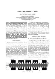A more simple generation of the error packets can be accomplished by generating the distance between two consecutive errors, solution which allows the generation of both packet errors and independent errors. The simulated transmission chain delivers a sequence of bits affected by errors as depicted in fig. 5.4. 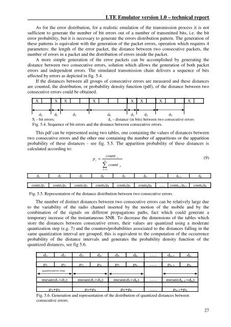If the distances between all groups of consecutive errors are measured and these distances are counted, the distribution, or probability density function (pdf), of the distance between two consecutive errors could be obtained. X X X X X X X X d2 d1 d3 d4 d1 d2 d3 X – bit errors; dx – distance (in bits) between two consecutive errors Fig. 5.4. Sequence of bit errors and the distance between consecutive errors. This pdf can be represented using two tables, one containing the values of distances between two consecutive errors and the other one containing the number of apparitions or the apparition probability of these distances - see fig. 5.5. The apparition probability of these distances is calculated according to: p i = n ∑ k = 1 count i count d1 d2 d3 d4 d5 d6 ...... dn-1 dn count1/p1 count2/p2 count3/p3 count4/p4 count5/p5 count6/p6 ...... countn-1/pn-1 countn/pn Fig. 5.5. Representation of the distance distribution between two consecutive errors. The number of distinct distances between two consecutive errors can be relatively large due to the variability of the radio channel inserted by the motion of the mobile and by the combination of the signals on different propagations paths, fact which could generate a temporary increase of the instantaneous SNR. To decrease the dimensions of the tables which store the distances between consecutive errors, their values are quantized using a moderate quantization step (e.g. 7) and the counters/probabilities associated to the distances falling in the same quantization interval are grouped; this is equivalent to the computation of the occurrence probability of the distance intervals and generates the probability density function of the quantized distances, see fig 5.6. d1 d2 d3 d4 d5 d6 ...... dn-1 dn p1 p2 p3 p4 p5 p6 ...... pn-1 pn quantization step mean(d1÷d2) mean(d3÷d4) mean(d5÷d6) ...... mean(dn-1÷dn) p1+p2 p3+p4 p5+p6 ...... pn-1+pn Fig. 5.6. Generation and representation of the distribution of quantized distances between consecutive errors. k (9) 27
TUCN – Data Transmission Laboratory Finally, two tables are stored for the representation of the error distribution, namely: the quantized values of the distances between two consecutive errors and the cumulated probability density function (cdf function), computed based on the pdf function. The cdf function can be used more easily for the generation of random variables distributed according a given pdf function. The generation of the error-sequences also requires the distribution of the number of errors on a TTI time interval. This distribution should be considered together with the number of transmitted bits in such an interval. At the output of the simulated transmission chain, besides the random variable describing the distances between consecutive errors, a bi-dimensional random variable which jointly describes the distribution of the numbers of bit errors/TTI and the distribution of the numbers of bits/TTI is also provided. These distributions can be described by the matrix presented in fig. 5.7. The indexing in the matrix is given by number of bit errors/TTI (on rows) and by the number of bits/TTI (on columns), and the positions inside the matrix give the number of occurrences of a certain combination (pairs of counters of numbers of errors/TTI and bits/TTI). The matrix structure presented in figure 5.7 is not worth to be used as such to generate the two combined random variable, due to two reasons: a lot of positions of the matrix are empty (some pairs no. errors/TTI, bits/TTI have null occurrence probabilities); the generation of bidimensional random variables is more complicated and requires more processing time. For an easier generation of the above mentioned random variables, the matrix of fig. 5.7. is transformed into 3 tables, after the suppression of the zero-value positions. One table contains the no. of bit errors/TTI, the second table contains the no. bits/TTI, and the third table contains the numbers of the considered pairs. For a certain position in the matrix, the same position is used in each table to store the three mentioned values, as shown in figure 5.8., which illustrates the transformation of the matrix presented in fig. 5.7. To further decrease the numbers of positions in the three tables, a distance dt between two consecutive positions is defined according to relation (9). 28 no. errors/TTI a b c d e f g h bits/TTI i j k l m count j-a count l-a count i-b count m-c count i-d count k-d count j-e count k-e count l-e count m-e count i-g count l-g count j-h Fig. 5.7. Matrix structure which describes the bi-dimensional random variable no. errors/TTI and no. bits/TTI. i i i j j j k k l l l m m b d g a e h d e a e g c e cnti-b cnti-d cnti-g cntj-a cntj-e cntj-h cntk-d cntk-e cntl-a cntl-e cntl-g cntm-c cntm-e Fig. 5.8. Representation of the distribution of the bi-dimensional random variable no. errors/TTI - no. bits/TTI using a set of three tables. bits/TTI bit errors /TTI d t _ i = bit _ eri − bit _ eri −1 + biti − biti−1 (9) where i is a given position in the tables, bit_eri represents the number of bit errors on position i, and biti represents the number of bits on position i.
Page 1 and 2: LTE Emulator (downlink connection)
Page 3 and 4: TUCN - Data Transmission Laboratory
Page 27: TUCN - Data Transmission Laboratory

LTE Emulator

You also want an ePaper? Increase the reach of your titles

Delete template?

Save as template?