Thermal Analysis of a H1616 Shipping Container - prod.sandia.gov ...
Thermal Analysis of a H1616 Shipping Container - prod.sandia.gov ...
Thermal Analysis of a H1616 Shipping Container - prod.sandia.gov ...

Create successful ePaper yourself
Turn your PDF publications into a flip-book with our unique Google optimized e-Paper software.
SAND REPORT<br />
SAND2002-8511<br />
Unlimited Release<br />
November 2002<br />
<strong>Thermal</strong> <strong>Analysis</strong> <strong>of</strong> a <strong>H1616</strong> <strong>Shipping</strong><br />
<strong>Container</strong> in Hypothetical Accident<br />
Conditions<br />
J. T. Hollenshead<br />
Prepared by<br />
Sandia National Laboratories<br />
Albuquerque, New Mexico 87185 and Livermore, California 94550<br />
Sandia is a multiprogram laboratory operated by Sandia Corporation,<br />
a Lockheed Martin Company, for the United States Department <strong>of</strong><br />
Energy under Contract DE-AC04-94AL85000.<br />
Approved for public release; further dissemination unlimited.
Issued by Sandia National Laboratories, operated for the United States Department <strong>of</strong><br />
Energy by Sandia Corporation.<br />
NOTICE: This report was prepared as an account <strong>of</strong> work sponsored by an agency <strong>of</strong><br />
the United States Government. Neither the United States Government, nor any agency<br />
there<strong>of</strong>, nor any <strong>of</strong> their employees, nor any <strong>of</strong> their contractors, subcontractors, or their<br />
employees, make any warranty, express or implied, or assume any legal liability or responsibility<br />
for the accuracy, completeness, or usefulness <strong>of</strong> any information, apparatus,<br />
<strong>prod</strong>uct, or process disclosed, or represent that its use would not infringe privately<br />
owned rights. Reference herein to any specific commercial <strong>prod</strong>uct, process, or service<br />
by trade name, trademark, manufacturer, or otherwise, does not necessarily constitute<br />
or imply its endorsement, recommendation, or favoring by the United States Government,<br />
any agency there<strong>of</strong>, or any <strong>of</strong> their contractors or subcontractors. The views and<br />
opinions expressed herein do not necessarily state or reflect those <strong>of</strong> the United States<br />
Government, any agency there<strong>of</strong>, or any <strong>of</strong> their contractors.<br />
Printed in the United States <strong>of</strong> America. This report has been re<strong>prod</strong>uced directly from<br />
the best available copy.<br />
Available to DOE and DOE contractors from<br />
U.S. Department <strong>of</strong> Energy<br />
Office <strong>of</strong> Scientific and Technical Information<br />
P.O. Box 62<br />
Oak Ridge, TN 37831<br />
Telephone: (865) 576-8401<br />
Facsimile: (865) 576-5728<br />
E-Mail: reports@adonis.osti.<strong>gov</strong><br />
Online ordering: http://www.doe.<strong>gov</strong>/bridge<br />
Available to the public from<br />
U.S. Department <strong>of</strong> Commerce<br />
National Technical Information Service<br />
5285 Port Royal Rd<br />
Springfield, VA 22161<br />
DEPARTMENT OF ENERGY<br />
Telephone: (800) 553-6847<br />
Facsimile: (703) 605-6900<br />
E-Mail: orders@ntis.fedworld.<strong>gov</strong><br />
Online ordering: http://www.ntis.<strong>gov</strong>/ordering.htm<br />
• •<br />
UNITED STATES<br />
OF AMERICA
SAND2002-8511<br />
Unlimited Release<br />
Printed November 2002<br />
<strong>Thermal</strong> <strong>Analysis</strong> <strong>of</strong> a <strong>H1616</strong> <strong>Shipping</strong> <strong>Container</strong><br />
in Hypothetical Accident Conditions<br />
Jeromy Todd Hollenshead<br />
<strong>Thermal</strong>/Fluid Modeling Department<br />
Sandia National Laboratories<br />
Livermore, CA 94551-0969<br />
jtholle@<strong>sandia</strong>.<strong>gov</strong><br />
November 21, 2002<br />
Abstract<br />
The thermal response <strong>of</strong> the <strong>H1616</strong> transport container is simulated to demonstrate<br />
compliance with the Federal regulations for performance during hypothetical accident<br />
conditions (HAC). The goal is to show that tests conducted for the certification <strong>of</strong> the<br />
<strong>H1616</strong> shipping container provide conservatively high estimates <strong>of</strong> temperatures at key<br />
regions within the container. A one-dimensional computational model is developed to<br />
simulate the thermal response <strong>of</strong> the shipping container in cylindrical coordinates. The<br />
model assumes the container is axisymmetric and allows for variable thermal properties.<br />
The model is calibrated using temperature data obtained from two experimental thermal<br />
tests and is then used to evaluate the thermal response <strong>of</strong> the shipping container to<br />
several different scenarios that meet or exceed the Federal regulations. A pre-heating<br />
technique, which is used to simulate the thermal effects <strong>of</strong> a radioactive heat source<br />
within the container, is also evaluated.<br />
3
Intentionally Left Blank<br />
4
Contents<br />
1 Introduction . . . . . . . . . . . . . . . . . . . . . . . . . . . . . . . . . . . . . . . . . . . . . . . . . . . . . . . . . 7<br />
2 Model Development and Validation . . . . . . . . . . . . . . . . . . . . . . . . . . . . . . . . . . 9<br />
3 Model Calibration. . . . . . . . . . . . . . . . . . . . . . . . . . . . . . . . . . . . . . . . . . . . . . . . . . . . 13<br />
4 <strong>Analysis</strong> and Results . . . . . . . . . . . . . . . . . . . . . . . . . . . . . . . . . . . . . . . . . . . . . . . . . 21<br />
Simulation <strong>of</strong> <strong>Thermal</strong> Tests including an Internal Heat Source . . . . . . . . . . . . . . . . 21<br />
Simulation <strong>of</strong> <strong>Thermal</strong> Tests at an Elevated Cooling Temperature . . . . . . . . . . . . . 26<br />
Simulation <strong>of</strong> <strong>Thermal</strong> Tests undergoing Solar Insolation . . . . . . . . . . . . . . . . . . . . . 34<br />
5 Conclusions . . . . . . . . . . . . . . . . . . . . . . . . . . . . . . . . . . . . . . . . . . . . . . . . . . . . . . . . . . 41<br />
References . . . . . . . . . . . . . . . . . . . . . . . . . . . . . . . . . . . . . . . . . . . . . . . . . . . . . . . . . . . . . . 45<br />
Figures<br />
1 Idealized Cross Section <strong>of</strong> <strong>Shipping</strong> <strong>Container</strong>. . . . . . . . . . . . . . . . . . . . . . . . . . 8<br />
2 Experimentally Observed Temperature Histories during the C6 <strong>Thermal</strong> Test. 14<br />
3 Experimentally Observed Temperature History during the C9 <strong>Thermal</strong> Test. 14<br />
4 Calibration to the C6 <strong>Thermal</strong> Test using only the Heat Transfer Coefficients. 15<br />
5 Calibration to the C6 <strong>Thermal</strong> Test including Foam Fire Effects. . . . . . . . . . . 16<br />
6 <strong>Shipping</strong> <strong>Container</strong> and Shroud Placement during <strong>Thermal</strong> Tests. . . . . . . . . . 18<br />
7 Final Calibration Results using the C6 <strong>Thermal</strong> Test Data. . . . . . . . . . . . . . . 18<br />
8 Final Calibration Results using the C9 <strong>Thermal</strong> Test Data. . . . . . . . . . . . . . . 20<br />
9 Steady-State Temperature Pr<strong>of</strong>iles for Different Values <strong>of</strong> Internal Heat Flux. 23<br />
10 Initial Steady-State Temperature Distribution (C9SIM vs. HSSIM1). . . . . . . 23<br />
11 Temperature Histories for Simulated <strong>Thermal</strong> Tests (C9SIM vs. HSSIM1). . . 24<br />
12 Flange Temperatures for Simulated <strong>Thermal</strong> Tests (C9SIM vs. HSSIM1). . . . 24<br />
13 Temperature Differences for Simulated <strong>Thermal</strong> Tests (C9SIM vs. HSSIM1). 25<br />
14 Initial Steady-State Temperature Distribution (C9SIM vs. HSSIM2). . . . . . . 27<br />
15 Temperature Histories for Simulated <strong>Thermal</strong> Tests (C9SIM vs. HSSIM2). . . 27<br />
16 Flange Temperatures for Simulated <strong>Thermal</strong> Tests (C9SIM vs. HSSIM2). . . . 28<br />
17 Temperature Differences for Simulated <strong>Thermal</strong> Tests (C9SIM vs. HSSIM2). 28<br />
18 Temperature Histories for Simulated <strong>Thermal</strong> Tests (C9SIM vs. CTSIM1). . 29<br />
19 Flange Temperatures for Simulated <strong>Thermal</strong> Tests (C9SIM vs. CTSIM1). . . 29<br />
20 Temperature Differences for Simulated <strong>Thermal</strong> Tests (C9SIM vs. CTSIM1). 30<br />
21 Temperature Histories for Simulated <strong>Thermal</strong> Tests (C9SIM vs. CTSIM2). . 31<br />
22 Flange Temperatures for Simulated <strong>Thermal</strong> Tests (C9SIM vs. CTSIM2). . . 31<br />
23 Temperature Differences for Simulated <strong>Thermal</strong> Tests (C9SIM vs. CTSIM2). 32<br />
24 Temperature Histories for Simulated <strong>Thermal</strong> Tests (C9SIM vs. CTSIM3). . 33<br />
5
25 Flange Temperatures for Simulated <strong>Thermal</strong> Tests (C9SIM vs. CTSIM3). . . 33<br />
26 Temperature Differences for Simulated <strong>Thermal</strong> Tests (C9SIM vs. CTSIM3). 34<br />
27 Temperature Histories for Simulated <strong>Thermal</strong> Tests (C9SIM vs. ISSIM1). . . 35<br />
28 Flange Temperatures for Simulated <strong>Thermal</strong> Tests (C9SIM vs. ISSIM1). . . . 36<br />
29 Temperature Differences for Simulated <strong>Thermal</strong> Tests (C9SIM vs. ISSIM1). . 36<br />
30 Temperature Histories for Simulated <strong>Thermal</strong> Tests (C9SIM vs. ISSIM2). . . 37<br />
31 Flange Temperatures for Simulated <strong>Thermal</strong> Tests (C9SIM vs. ISSIM2). . . . 38<br />
32 Temperature Differences for Simulated <strong>Thermal</strong> Tests (C9SIM vs. ISSIM2). . 38<br />
33 Temperature Histories for Simulated <strong>Thermal</strong> Tests (C9SIM vs. ISSIM3). . . 40<br />
34 Flange Temperatures for Simulated <strong>Thermal</strong> Tests (C9SIM vs. ISSIM3). . . . 40<br />
35 Temperature Differences for Simulated <strong>Thermal</strong> Tests (C9SIM vs. ISSIM3). . 41<br />
Tables<br />
1 Layer Characteristics <strong>of</strong> the <strong>Shipping</strong> <strong>Container</strong>. . . . . . . . . . . . . . . . . . . . . . . . 8<br />
2 Selected Properties <strong>of</strong> Materials within the <strong>Shipping</strong> <strong>Container</strong>. . . . . . . . . . . . 10<br />
3 <strong>Thermal</strong> Properties <strong>of</strong> the Polyurethane Foam. . . . . . . . . . . . . . . . . . . . . . . . . . 10<br />
4 <strong>Thermal</strong> Properties <strong>of</strong> the Packing Material. . . . . . . . . . . . . . . . . . . . . . . . . . . . 11<br />
5 <strong>Thermal</strong> Properties <strong>of</strong> the <strong>Thermal</strong> Barrier. . . . . . . . . . . . . . . . . . . . . . . . . . . . 11<br />
6 <strong>Thermal</strong> Properties <strong>of</strong> 304 Stainless Steel. . . . . . . . . . . . . . . . . . . . . . . . . . . . . . 11<br />
7 Final Model Parameters determined through Calibration. . . . . . . . . . . . . . . . . 19<br />
8 System Properties Predicted from <strong>Thermal</strong> Calibration Tests. . . . . . . . . . . . . 19<br />
9 Description and Results <strong>of</strong> the C9 Simulation Scenarios. . . . . . . . . . . . . . . . . . 39<br />
6
<strong>Thermal</strong> <strong>Analysis</strong> <strong>of</strong> a <strong>H1616</strong><br />
<strong>Shipping</strong> <strong>Container</strong> in Hypothetical<br />
Accident Conditions<br />
1 Introduction<br />
During the spring <strong>of</strong> 2001, personnel from organization 8243 were finalizing the Safety<br />
<strong>Analysis</strong> Report for Packaging (SARP) for the <strong>H1616</strong> shipping container when it was observed<br />
that the hypothetical accident condition (HAC) scenario as defined in the Federal<br />
requirements document [2] had not been tested for correctly. The requirements call for the<br />
container to be placed in a high temperature environment where the temperature exceeds<br />
1475 ◦ F, such as in a pool fire or heat radiation facility, for thirty minutes. The requirements<br />
then specify that the container should be placed in an ambient temperature <strong>of</strong> 100 ◦ F and<br />
exposed to twelve hours <strong>of</strong> solar insolation followed by twelve hours without insolation. This<br />
pattern <strong>of</strong> solar insolation should be repeated until the temperature reaches steady-state.<br />
In the actual experimental tests conducted for the SARP, containers were placed in<br />
a high temperature environment for thirty minutes, but then were removed and allowed<br />
to cool at an ambient temperature <strong>of</strong> approximately 40 ◦ F and without solar insolation.<br />
Additionally, the experiments were conducted on shipping containers without an internal<br />
heat source. In actual conditions, a heat generation source <strong>of</strong> up to 6.5 Watts would be<br />
present within the container. In order to simulate the thermal effects <strong>of</strong> a heat source,<br />
the empty shipping containers were heated to an elevated temperature <strong>of</strong> 160 ◦ F before the<br />
thermal tests were conducted.<br />
The goal <strong>of</strong> this project is to show compliance <strong>of</strong> the <strong>H1616</strong> shipping container with<br />
Federal regulations by simulating the container’s thermal response under the specified conditions.<br />
A one-dimensional finite difference model <strong>of</strong> the shipping container is developed in<br />
cylindrical coordinates. The model assumes the container is axisymmetric and allows for<br />
variable thermal properties in the radial direction. The model is first calibrated using the<br />
data obtained from thermal experiments and then used to demonstrate that the thermal<br />
performance <strong>of</strong> the shipping container meets or exceeds the requirements. The maximum<br />
temperature reached by the O-ring located near the flange <strong>of</strong> the containment vessel is<br />
used as the key measure <strong>of</strong> the systems thermal response. The following analysis evaluates<br />
whether pre-heating shipping containers before the thermal experiments suitably takes into<br />
account the lack <strong>of</strong> the heat generation source on the maximum temperature reached by this<br />
O-ring. The analysis also evaluates the difference in the maximum temperature reached at<br />
the O-ring between the conditions as tested (cooling at 40 ◦ F with no solar insolation) and<br />
those specified by the Federal requirements (cooling at 100 ◦ F with solar insolation).<br />
This report is divided into sections. Section 2 describes the geometry <strong>of</strong> the shipping<br />
7
Steel<br />
Packing Material<br />
Steel<br />
r<br />
Reservior O-ring/Flange<br />
Steel<br />
Polyfoam<br />
Ceramic<br />
Steel<br />
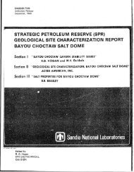
Figure 1. Idealized Cross Section <strong>of</strong> <strong>Shipping</strong> <strong>Container</strong> (Top View).<br />
container and outlines the methodology used to develop and validate the numerical model.<br />
Section 3 discusses the calibration <strong>of</strong> the thermal model using temperature data from two<br />
thermal experiments. Section 4 then details the simulation <strong>of</strong> thermal tests for several<br />
different scenarios and discusses the results. The results are then summarized in Section 5.<br />
Table 1. Layer Characteristics <strong>of</strong> the <strong>Shipping</strong> <strong>Container</strong>.<br />
Thickness (inch) Radius (inch) Thickness (m) Radius (m) Material<br />
1.500 1.500 0.038100 0.038100 Air<br />
0.250 1.750 0.006350 0.044450 Stainless Steel<br />
4.305 6.055 0.109347 0.153797 Packing Material<br />
0.135 6.190 0.003429 0.157226 Stainless Steel<br />
0.030 6.220 0.000762 0.157988 Stainless Steel<br />
0.970 7.190 0.024638 0.182626 Polyurethane Foam<br />
0.500 7.690 0.012700 0.195326 <strong>Thermal</strong> Barrier<br />
0.048 7.738 0.001219 0.196545 Stainless Steel<br />
8
2 Model Development and Validation<br />
The <strong>H1616</strong> transport container consists <strong>of</strong> an eighteen gauge insulated stainless steel drum<br />
approximately 21.5 inches in length and 16.5 inches in diameter. At the center <strong>of</strong> the<br />
container is a stainless steel vessel known as the reservoir that is spherical and has an approximate<br />
diameter <strong>of</strong> 3.0 inches. When in use, this inner vessel contains a radioactive<br />
material that <strong>prod</strong>uces decay heat which contributes to the thermal loading <strong>of</strong> the system.<br />
Surrounding the reservoir is a thick layer <strong>of</strong> packing material made from aluminum tubing.<br />
Both the reservoir and packing material are contained within a 304 stainless steel containment<br />
vessel. The containment vessel is placed within the outer stainless steel drum and the<br />
air space between is filled with a polyurethane foam. A one half inch thick layer <strong>of</strong> ceramic<br />
fiber lines the inside <strong>of</strong> the outer steel drum to provide an additional thermal barrier.<br />
Although the geometry <strong>of</strong> the shipping container is known completely, the current analysis<br />
describes the flow <strong>of</strong> heat through the container as a one-dimensional axisymmetric<br />
problem in cylindrical coordinates. While this greatly simplifies the problem, it also increases<br />
the level <strong>of</strong> uncertainty associated with the results. Increasing the complexity <strong>of</strong><br />
the shipping container geometry would help to decrease the level <strong>of</strong> uncertainly in the results,<br />
but would require additional time and funding which are not available. It is therefore<br />
assumed the thermal description <strong>of</strong> the problem is suitable and adequately describes the<br />
geometry and physical processes <strong>of</strong> interest. Figure 1 shows the idealized cross-section <strong>of</strong><br />
the shipping container in cylindrical coordinates. The various layers that make up the<br />
container, their radial thicknesses, and the distance <strong>of</strong> each layer from the center <strong>of</strong> the<br />
container are shown in Table 1.<br />
The origin <strong>of</strong> the coordinate system is chosen to be the at the center <strong>of</strong> the reservoir<br />
within the shipping container. The flow <strong>of</strong> heat is described using the differential energy<br />
balance equation[3] :<br />
<br />
1 ∂<br />
r<br />
kr ∂T<br />
∂r<br />
∂r<br />
<br />
∂T<br />
+ q = ρCp , (1)<br />
∂t<br />
where k is the thermal conductivity, q is a volumetric heat generation term, and Cp is the<br />
specific heat at constant pressure. The associated initial temperature distribution:<br />
and boundary conditions on the inside(a):<br />
and outside(b) <strong>of</strong> the shipping container:<br />
T (0, x) = g(x), (2)<br />
−k ∂T<br />
∂r |a = ha (Ta − T∞) − qa, (3)<br />
−k ∂T<br />
∂r |b<br />
<br />
= hb (Tb − T∞) − qb + ɛσ T 4 b − T 4 <br />
∞ , (4)<br />
9
Table 2. Selected Properties <strong>of</strong> Materials within the <strong>Shipping</strong> <strong>Container</strong>.<br />
Material Density (kg/m 3 ) Solar Absorptivity<br />
Stainless Steel 8083 0.37<br />
Packing Material 401 –<br />
Polyurethane Foam 264 –<br />
Ceramic <strong>Thermal</strong> Barrier 60 –<br />
Table 3. <strong>Thermal</strong> Properties <strong>of</strong> the Polyurethane Foam.<br />
Temperature (C) Cp (J/g ◦ C) k (Btu in. / hr ft 2 ◦ F)<br />
25 1.35 0.34<br />
50 1.83 –<br />
100 2.46 –<br />
150 3.12 –<br />
are also required to determine the temperature distribution within the container at any time.<br />
During the simulation, the values <strong>of</strong> the parameters in Eqs. (3) and (4) are modified to<br />
simulate conditions specified by the Federal requirements. These equations are discretized<br />
using a finite volume scheme. The thermal properties <strong>of</strong> materials within the shipping<br />
container vary as a function <strong>of</strong> temperature and are tabulated in the original SARP report<br />
[6] at a number <strong>of</strong> discrete temperatures. These values are used to linearly interpolate<br />
property values at temperatures between the reported values. Properties at temperatures<br />
outside the range <strong>of</strong> the provided values are evaluated at the highest or lowest temperature<br />
available. Tables 2 – 4 show the thermal and other relevant properties <strong>of</strong> interest for the<br />
materials used within the shipping container.<br />
A computational program written in FORTRAN is used to solve the equations describing<br />
flow using a scheme that is explicit in time and implicit in position. This formulation yields<br />
a tri-diagonal matrix that is solved using the Thomas algorithm [5] at each time step.<br />
The total number <strong>of</strong> volume elements in the radial direction is increased to discretize the<br />
spatial domain into smaller and smaller elements until the solution converges. The final<br />
model is comprised <strong>of</strong> 1000 volume elements. The uniform time step used in the program<br />
is also systematically reduced until no appreciable change in the solution is observed. At<br />
each time step, physical properties are evaluated iteratively, starting with the temperature<br />
determined at the last time step and continuing until the temperatures used to calculate<br />
the physical properties converge to the temperature pr<strong>of</strong>ile at the new time step. The<br />
developed model is validated by comparing the steady-state numerical solution with an<br />
analytical solution determined using a thermal resistance model [3]. Once the model is<br />
validated, thermal properties within the model are determined from experimental thermal<br />
tests. The calibration methodology is described in the following section.<br />
10
Table 4. <strong>Thermal</strong> Properties <strong>of</strong> the Packing Material.<br />
Temperature (C) Cp (kJ/Kg ◦ K) k (W / m ◦ F)<br />
27 0.96 0.35<br />
Table 5. <strong>Thermal</strong> Properties <strong>of</strong> the <strong>Thermal</strong> Barrier.<br />
Temperature (F) Cp (Btu/ lb ◦ F) k (Btu in. / hr ft 2 ◦ F)<br />
400 0.39 0.235<br />
800 0.52 0.261<br />
1200 0.67 0.274<br />
1600 0.84 0.283<br />
Table 6. <strong>Thermal</strong> Properties <strong>of</strong> 304 Stainless Steel.<br />
Temperature (K) Cp (J/kg K) k (W/m K) Emissivity (ɛ)<br />
100 272 9.2 –<br />
200 402 12.6 –<br />
300 477 14.9 –<br />
400 515 16.6 –<br />
600 557 19.8 –<br />
800 582 22.6 0.33<br />
1000 611 25.4 0.40<br />
1200 640 28.0 –<br />
11
Intentionally Left Blank<br />
12
3 Model Calibration<br />
In order to ensure the thermal performance <strong>of</strong> the <strong>H1616</strong> shipping container satisfied the<br />
Federal requirements for hypothetical accident conditions (HAC), several field experiments<br />
were conducted for the previous SARP in both radiant heat facilities and in fuel pool fires.<br />
In the current analysis, data from two thermal tests conducted in radiant heat facilities is<br />
used to calibrate the numerical model. These data are used to estimate the parameters,<br />
such as the heat transfer coefficients (ha,hb), that appear in Eqs. (3) and (4).<br />
Before the heating portion <strong>of</strong> the thermal test is initiated, the containers are pre-heated<br />
in a 160 ◦ F oven until steady-state conditions are reached. This procedure is designed to<br />
compensate for the elevated temperatures that would be present in a filled container due to<br />
the internal heat source. The containers are then exposed to temperatures over 1475 ◦ F for<br />
approximately thirty minutes. The ambient temperature is then reduced and the container<br />
is allowed to cool and come to thermal equilibrium with its surroundings. Thermocouples<br />
placed on the sides <strong>of</strong> the drum and at various locations <strong>of</strong> interest within the container<br />
itself continuously record temperatures throughout the thermal test. Additionally, blackout<br />
indicators, which turn black once they are exposed to a specified maximum temperature,<br />
are located in several locations throughout the container during testing. A more complete<br />
description <strong>of</strong> the experimental procedures and a complete record <strong>of</strong> additional tests that<br />
were conducted may be found in the original SARP report [6].<br />
Figure 2 shows temperature data from the C6 test, the first thermal test. Since the<br />
actual electronic data files are not available, discrete temperature values from both the<br />
shroud and the flange are read from figures contained within the SARP report [6]. The<br />
observed flange temperatures are shown in green and the shroud temperatures are shown<br />
in red. In the C6 thermal experiment, radiant heat lamps are switched on at around five<br />
minutes into the experiment, and the shroud temperature quickly rises above the required<br />
temperature <strong>of</strong> 1475 ◦ F to 1525 ◦ F. After thirty minutes the heat lamps are turned <strong>of</strong>f and the<br />
system is allowed to cool at the ambient temperature, which is assumed to be around 40 ◦ F.<br />
The maximum flange temperature recorded in the experiment is 344.7 ◦ F. During the C9<br />
thermal test, only the shroud temperature history, which is shown in Figure 3, is recorded.<br />
The test is conducted in essentially the same fashion as the C6 test with the exception than<br />
the shroud reaches a temperature <strong>of</strong> 1850 ◦ F. The maximum recorded flange temperature is<br />
465 ◦ F.<br />
The model is first calibrated using the data from the C6 thermal test because temperature<br />
pr<strong>of</strong>iles are available for both the shroud and O-ring/flange regions. Initially, only the<br />
values <strong>of</strong> the ambient heat transfer coefficients, ha and hb in Eqs. (3) and (4), are modified.<br />
A trial and error method is used to obtain the best match between the model prediction<br />
and the experimentally observed temperatures. The best predictions obtained by modifying<br />
only the heat transfer coefficients are shown in Figure 4. Here, the model predicts that the<br />
shroud cools <strong>of</strong>f much more rapidly than what is observed experimentally. Additionally, the<br />
13
Temperature (F)<br />
1600<br />
1400<br />
1200<br />
1000<br />
800<br />
600<br />
400<br />
200<br />
Shroud Temperature (C6 <strong>Thermal</strong> Test)<br />
Flange Temperature (C6 <strong>Thermal</strong> Test)<br />
0<br />
0 20 40 60 80 100 120 140 160 180 200<br />
Time (min)<br />
Figure 2. Experimentally Observed Temperature Histories during the C6 <strong>Thermal</strong> Test.<br />
Temperature (F)<br />
2000<br />
1500<br />
1000<br />
500<br />
0<br />
0 20 40 60 80 100 120 140 160 180 200<br />
Time (min)<br />
Shroud Temperature (C9 <strong>Thermal</strong> Test)<br />
Figure 3. Experimentally Observed Temperature History during the C9 <strong>Thermal</strong> Test.<br />
14
Temperature (F)<br />
1600<br />
1400<br />
1200<br />
1000<br />
800<br />
600<br />
400<br />
200<br />
Shroud Temperature (C6 <strong>Thermal</strong> Test)<br />
Flange Temperature (C6 <strong>Thermal</strong> Test)<br />
Shroud Temperature (Model Prediction)<br />
Flange Temperature (Model Prediction)<br />
0<br />
0 20 40 60 80 100 120 140 160 180 200<br />
Time (min)<br />
Figure 4. Calibration to the C6 <strong>Thermal</strong> Test using only the Heat Transfer Coefficients.<br />
predicted maximum flange temperature is approximately 270 ◦ F, significantly less than the<br />
observed value <strong>of</strong> 344.7 ◦ F.<br />
It was determined that in order for the predicted pr<strong>of</strong>iles to match the experimentally<br />
observed values, an additional heat generation source is required within the system. After<br />
additional discussions with several people who observed the thermal test, it is determined<br />
that at the conclusion <strong>of</strong> the thermal experiments, the polyurethane foam surrounding the<br />
inner containment vessel is typically burning. It is observed that the foam first expands<br />
and then contracts so that it effectively disintegrates into a small amount <strong>of</strong> material at the<br />
bottom <strong>of</strong> the shipping container. This observation supports the idea that temperatures<br />
reached within the polyurethane foam layer are high enough to catch the foam on fire<br />
during the heating portion <strong>of</strong> the experiment. The heat released during this process serves<br />
as an additional heat source. In addition, the thermal properties <strong>of</strong> the foam may change<br />
substantially after being burned. If the foam completely decomposes within the container, it<br />
may also be necessary to allow for thermal radiation across this newly formed air interface.<br />
However, for the present analysis, the foam is assumed not to disintegrate and form a<br />
void space. Additionally, brief experimentation with the thermal properties <strong>of</strong> the foam<br />
during the fire shows no significant change to the predicted temperatures. Consequently,<br />
the thermal properties <strong>of</strong> the foam as a function <strong>of</strong> temperature are not modified after the<br />
foam fire. While it would be beneficial to investigate the manner in which the foam burns<br />
15
Temperature (F)<br />
1600<br />
1400<br />
1200<br />
1000<br />
800<br />
600<br />
400<br />
200<br />
Shroud Temperature (C6 <strong>Thermal</strong> Test)<br />
Flange Temperature (C6 <strong>Thermal</strong> Test)<br />
Shroud Temperature (Model Prediction)<br />
Flange Temperature (Model Prediction)<br />
0<br />
0 20 40 60 80 100 120 140 160 180 200<br />
Time (min)<br />
Figure 5. Calibration to the C6 <strong>Thermal</strong> Test including Foam Fire Effects.<br />
and how its properties are modified because <strong>of</strong> the fire, the urgency <strong>of</strong> the final results<br />
require that crude assumptions be made on the effects <strong>of</strong> the internal polyurethane fire on<br />
the thermal response <strong>of</strong> the shipping container. In the approach taken, the burning foam<br />
is included as an energy source that heats the system between designated start and end<br />
times which are determined by trial and error. In future studies it would be beneficial to<br />
determine the temperature at which the foam starts to burn and associate the start <strong>of</strong> the<br />
foam fire with the time this temperature is reached.<br />
The amount <strong>of</strong> heat generated by the foam fire is determined by multiplying the total<br />
heat <strong>of</strong> combustion, Hc ( 7.22 MJ/kg [1]), by the density, ρf <strong>of</strong> the polyurethane foam.<br />
This yields the number <strong>of</strong> Joules released per volume if the foam burns completely. To take<br />
into account incomplete combustion, a parameter known as the fire factor, χ, is introduced.<br />
This factor may be interpreted as the percentage <strong>of</strong> the foam that burns in the time between<br />
a specified fire start and end time. The total number <strong>of</strong> Watts generated per volume during<br />
the foam fire is then given as:<br />
qfoam = χ Hcρf<br />
, (5)<br />
te − ts<br />
where the fire factor, χ, and fire start and end times, ts and te, are additional parameters<br />
to be estimated.<br />
The results <strong>of</strong> calibrating the numerical model using these additional parameters are<br />
16
shown in Figure 5 using the parameters specified in Table 7. The predicted flange temperatures<br />
are now found to be considerably closer to the experimentally observed values than<br />
the previous predictions made without considering the foam fire. The maximum flange temperature<br />
is estimated to be 335.5 ◦ F which is much closer to the observed value <strong>of</strong> 344.7 ◦ F<br />
than the 270 ◦ F value determined earlier. However, while the predicted shroud temperatures<br />
are closer to the observed values, there is not a suitable match. The effects <strong>of</strong> the foam<br />
fire are seen to more directly affect the temperature at the flange than the temperature at<br />
the shroud. This is expected since the flange is physically closer to the foam fire, being<br />
separated only by a stainless steel layer which has a high thermal conductivity.<br />
The predicted shroud temperature is found to be most sensitive to the emissivity value<br />
used for the outer steel drum. The best match between predicted and observed values <strong>of</strong><br />
both the flange temperature and shroud temperature pr<strong>of</strong>iles is obtained when it is assumed<br />
that the emissivity <strong>of</strong> the outer steel container changes after the fire. An emissivity factor<br />
that is 20% <strong>of</strong> the tabulated value gives the best match to experimental data. This value is<br />
considerably smaller than expected. After completing the analysis, it is determined that the<br />
shroud is not the outer skin <strong>of</strong> the shipping container as assumed. Instead, the shroud is a<br />
large metal plate that surrounds the shipping containers during the thermal tests. A sample<br />
experimental layout is shown in Figure 6. The radiant heat lamps are focused on these<br />
stainless steel metal shrouds to more evenly distribute the energy to the shipping containers.<br />
The thermal model does not explicitly take into account the relationship between the metal<br />
shroud, the shipping container, and the air between them. Instead, it is assumed that<br />
the determined emissivity value is actually an effective property that implicitly takes into<br />
account these effects. Although this practice is not standard and leads to an uncharacteristic<br />
emissivity, it is not anticipated that it will impact the conclusions <strong>of</strong> the current analysis<br />
as we are primarily concerned with the the temperature history at the O-ring and flange<br />
which lie within the container.<br />
The temperature history resulting from the final calibration to the C6 thermal experiment<br />
is shown in Figure 7. The maximum flange temperature <strong>of</strong> 345 ◦ F is essentially the<br />
same as the observed value <strong>of</strong> 344.7 ◦ F. During the calibration <strong>of</strong> the model with the thermal<br />
tests, no solar flux effects are included since initial tests indicated that the addition<br />
<strong>of</strong> a solar flux effects results in temperatures much higher than those observed during the<br />
experiment. It is concluded that there are minimal effects due to solar heat flux during the<br />
actual thermal experiments.<br />
Once the model is successfully calibrated using the data from the C6 thermal test, it is<br />
desired to use the same model parameters to match the C9 thermal test data. Although<br />
using the parameters determined from the C6 thermal test yield a qualitative match <strong>of</strong> the<br />
temperature history to the C9 data, it is necessary to make additional modifications to<br />
obtain a satisfactory match. The parameters determined in the C9 calibration are shown in<br />
Table 7 and the comparison to the thermal experiment is shown in Figure 8. The maximum<br />
flange temperature reached is 465.7 ◦ F which corresponds closely to the observed value <strong>of</strong><br />
465 ◦ F. The most substantial change between the parameters when calibrating using the two<br />
17
Heat Lamp<br />
shipping<br />
container<br />
Heat Lamp<br />
shipping<br />
container<br />
Heat Lamp<br />
Shroud Shroud<br />
Heat Lamp<br />
Figure 6. <strong>Shipping</strong> <strong>Container</strong> and Shroud Placement during <strong>Thermal</strong> Tests.<br />
Temperature (F)<br />
1600<br />
1400<br />
1200<br />
1000<br />
800<br />
600<br />
400<br />
200<br />
Shroud Temperature (C6 <strong>Thermal</strong> Test)<br />
Flange Temperature (C6 <strong>Thermal</strong> Test)<br />
Shroud Temperature (Model Prediction)<br />
Flange Temperature (Model Prediction)<br />
0<br />
0 20 40 60 80 100 120 140 160 180 200<br />
Time (min)<br />
Figure 7. Final Calibration Results using the C6 <strong>Thermal</strong> Test Data.<br />
18
Table 7. Final Model Parameters determined through Calibration.<br />
C6 <strong>Thermal</strong> Test C9 <strong>Thermal</strong> Test<br />
Foam Fire Start (ts) 20 minutes 30 minutes<br />
Foam Fire End (te) 40 minutes 50 minutes<br />
Foam Fire Factor (χ) 0 .14 0.32<br />
Heat Transfer Coefficient (hb) 5.5 W/m 2 ◦ K 7.0 W/m 2◦ K<br />
Emissivity (% <strong>of</strong> tabulated ) (ɛ) 0.20 0.20<br />
Cooling Air Temp 40 ◦ F 40 ◦ F<br />
Table 8. System Properties Predicted from <strong>Thermal</strong> Calibration Tests.<br />
C6 Test C9 Test<br />
Foam Fire Duration 20 minutes 20 minutes<br />
Foam Fire Heat Generation 117,628 W/m 3 260,460 W/m 3<br />
Max. Flange Temp. ( Predicted) 345.0 ◦ F 465.7 ◦ F<br />
Max. Flange Temp. ( Experimental) 344.7 ◦ F 465.0 ◦ F<br />
thermal experiments is seen in fire factor, χ. The fire factor determined in the C9 thermal<br />
test is 0.32, a value larger than the value <strong>of</strong> 0.14 determined in the C6 thermal test. This<br />
implies that the foam released more energy in the C9 test which may be a consequence <strong>of</strong><br />
the higher temperature reached by the polyurethane foam layer due to the higher shroud<br />
temperature.<br />
19
Temperature (F)<br />
2000<br />
1500<br />
1000<br />
500<br />
Shroud Temperature (C9 <strong>Thermal</strong> Test)<br />
Shroud Temperature (Model Prediction)<br />
Flange Temperature (Model Prediction)<br />
0<br />
0 20 40 60 80 100 120 140 160 180 200<br />
Time (min)<br />
Figure 8. Final Calibration Results using the C9 <strong>Thermal</strong> Test Data.<br />
20
4 <strong>Analysis</strong> and Results<br />
Once the model is calibrated using the experimental thermal tests, it is possible to simulate<br />
the thermal tests and evaluate several different scenarios. In the following sections,<br />
temperature histories associated with each scenario are determined and are compared with<br />
a simulation <strong>of</strong> the C9 thermal test. The first section simulates the thermal response <strong>of</strong><br />
a pre-heated shipping container and compares it with a simulation that explicitly models<br />
a heat source in the center <strong>of</strong> the shipping container. The second section describes simulations<br />
<strong>of</strong> the thermal tests at the ambient conditions specified by the Federal documents.<br />
The last section describes simulations <strong>of</strong> thermal tests at the ambient conditions specified<br />
by the Federal documents and which include the effects <strong>of</strong> solar insolation. A summary <strong>of</strong><br />
the thermal conditions used in each <strong>of</strong> the scenarios is shown in Table 9.<br />
Simulation <strong>of</strong> <strong>Thermal</strong> Tests including an Internal Heat Source<br />
<strong>Thermal</strong> testing <strong>of</strong> the <strong>H1616</strong> shipping containers is necessary to demonstrate that the containers<br />
are able to satisfactory withstand thermal environments that may be present during<br />
accident conditions. The containers are designed to transport a radioactive material which<br />
may continuously generate a maximum <strong>of</strong> 6.5 Watts. Because <strong>of</strong> the dangers associated<br />
with handling radioactive materials, it is not possible to test filled containers. Thus, the<br />
elevated temperature distribution within a filled container, which is due to the presence<br />
<strong>of</strong> the radioactive material, is taken into account thermally by pre-heating empty shipping<br />
containers to an elevated temperature. This pre-heat temperature is typically chosen to be<br />
greater than the highest expected temperature found in a filled container at steady-state<br />
conditions. While this technique adequately takes into account the higher initial condition,<br />
it does not simulate the generation <strong>of</strong> heat throughout the entire thermal tests. Thus the<br />
effectiveness <strong>of</strong> the technique diminishes as the test proceeds. One question to be answered<br />
by this analysis is whether the maximum O-ring/flange temperature measured using the<br />
pre-heating technique provides a conservatively high measure <strong>of</strong> the maximum O-ring/flange<br />
temperature that would be observed in a filled shipping container.<br />
In order to evaluate the pre-heating technique, the C9 thermal test is first simulated<br />
as performed in the field. The results <strong>of</strong> this simulation serve as a point <strong>of</strong> reference with<br />
which to compare additional simulations. This simulation, which is labeled the C9SIM<br />
scenario, involves first pre-heating an empty shipping container in a 160 ◦ F environment<br />
until thermal equilibrium is established. The container is then exposed to a powerful heat<br />
source which quickly brings the outside temperature <strong>of</strong> the shipping container to 1825 ◦ F.<br />
After thirty minutes <strong>of</strong> exposure, the powerful heat source is removed and the container<br />
is allowed to cool in a 40 ◦ F environment. After the C9 thermal test has been simulated,<br />
the determined temperatures are compared with temperatures determined in additional<br />
simulations that take into account a number <strong>of</strong> different conditions. In this manner, it is<br />
21
possible to evaluate the thermal effects <strong>of</strong> including an internal heat source, increasing the<br />
ambient cooling temperature, and/or taking into account solar insolation. The ability for<br />
the C9 thermal test to predict a conservatively high maximum flange temperature for each<br />
<strong>of</strong> the various scenarios is determined by ensuring that the maximum flange temperature<br />
measured in the C9 thermal test is greater than the maximum flange temperature predicted<br />
in the remaining scenarios.<br />
The first group <strong>of</strong> scenarios to be simulated repeat the C9 thermal test without the preheating<br />
step and include the effects <strong>of</strong> an internal heat source. Before this heat source can<br />
be simulated, it is necessary to determine a suitable value for the heat flux to be applied to<br />
the interior <strong>of</strong> the shipping container. The reservoir that contains the heat source releases<br />
a maximum <strong>of</strong> 6.5 W. It is approximately spherical and is located at the center <strong>of</strong> the<br />
shipping container. Because each <strong>of</strong> the layers in the shipping container is modeled as a<br />
cylinder, it is necessary to convert the heat source into an appropriate flux. There are<br />
two possible approaches. The first determines the heat flux across the surface area <strong>of</strong> the<br />
reservoir sphere and then uses the same value over the surface <strong>of</strong> a cylinder. This provides<br />
a worst case situation and results in a heat flux <strong>of</strong> 356.33 W/m 2 . Over a cylinder <strong>of</strong> length<br />
one meter, this corresponds to 85.3 W, a value much larger than the spherical value <strong>of</strong> 6.5<br />
Watts. Simulating the C9 thermal test using this value results in temperatures much higher<br />
than expected. A second approach that determines the heat flux required for a one meter<br />
cylinder to <strong>prod</strong>uce 6.5 Watts yields a value <strong>of</strong> 27.15 W/m 2 .<br />
The most appropriate value for the heat source is determined by simulating a steadystate<br />
thermal experiment that was conducted using resistance heating for the original SARP<br />
report [6]. Here a shipping container with a 6.5 Watt heat source is allowed to come to<br />
thermal equilibrium in a 100 ◦ F environment. The maximum observed temperature during<br />
the experiment is 148 ◦ F which is reached at the center reservoir. The developed model<br />
is used to simulate this steady-state thermal experiment and determine the temperature<br />
distributions associated with three different heat flux values, 27.15 W/m 2 , 60 W/m 2 , and<br />
120 W/m 2 . Figure 9 shows the determined steady-state temperature pr<strong>of</strong>iles as a function<br />
<strong>of</strong> radial position. The temperature distribution is axisymmetric and the x-axis indicates<br />
the distance from the center <strong>of</strong> the shipping container. For each flux, the highest temperature<br />
is predicted at the reservoir (around 0.04 meters). The temperature variations as a<br />
function <strong>of</strong> position seen in Figure 9 are due to the various materials that comprise the<br />
shipping container. The area <strong>of</strong> interest, the location <strong>of</strong> the flange and O-ring, is located at<br />
approximately 0.157 meters from the center <strong>of</strong> the container. Based on the results <strong>of</strong> the<br />
simulations, a heat flux <strong>of</strong> 80 W/m 2 is seen to provide a maximum temperature <strong>of</strong> 150 ◦ F<br />
which is suitably close the the observed value <strong>of</strong> 148 ◦ F. Using this flux, the predicted Oring/flange<br />
temperature at steady-state is approximately 128F ◦ which is 28F ◦ greater than<br />
the ambient temperature. In additional to evaluating the 80 W/m 2 flux, a conservatively<br />
high value <strong>of</strong> 120 W/m 2 is also examined.<br />
The developed model is now used to estimate the temperature history <strong>of</strong> a filled container.<br />
The influence <strong>of</strong> the radioactive material at the center <strong>of</strong> the shipping container is<br />
22
Temperature (F)<br />
180<br />
170<br />
160<br />
150<br />
140<br />
130<br />
120<br />
110<br />
100<br />
0.02 0.04 0.06 0.08 0.1 0.12 0.14 0.16 0.18 0.2<br />
Radial Length (meters)<br />
30 Watt/meter^2 Heat Source<br />
60 Watt/meter^2 Heat Source<br />
80 Watt/meter^2 Heat Source<br />
120 Watt/meter^2 Heat Source<br />
Figure 9. Steady-State Temperature Pr<strong>of</strong>iles for Different Values <strong>of</strong> Internal Heat Flux.<br />
Temperature (F)<br />
170<br />
160<br />
150<br />
140<br />
130<br />
120<br />
110<br />
100<br />
0.02 0.04 0.06 0.08 0.1 0.12 0.14 0.16 0.18 0.2<br />
Radial Length (meters)<br />
Initial Temperature (C9SIM)<br />
Initial Temperature (HSSIM1)<br />
Figure 10. Initial Steady-State Temperature Distribution (C9SIM vs. HSSIM1).<br />
23
Temperature (F)<br />
2000<br />
1800<br />
1600<br />
1400<br />
1200<br />
1000<br />
800<br />
600<br />
400<br />
200<br />
0<br />
0 20 40 60 80 100 120 140 160 180 200<br />
Time (min)<br />
Shroud Temperature (HSSIM1)<br />
Flange Temperature (HSSIM1)<br />
Shroud Temperature (C9SIM)<br />
Flange Temperature (C9SIM)<br />
Figure 11. Temperature Histories for Simulated <strong>Thermal</strong> Tests (C9SIM vs. HSSIM1).<br />
Temperature (F)<br />
500<br />
450<br />
400<br />
350<br />
300<br />
250<br />
200<br />
150<br />
100<br />
0 100 200 300 400 500 600 700 800 900 1000<br />
Time (min)<br />
Flange Temperature (HSSIM1)<br />
Flange Temperature (C9SIM)<br />
Figure 12. Flange Temperatures for Simulated <strong>Thermal</strong> Tests (C9SIM vs. HSSIM1).<br />
24
Temperature (F)<br />
60<br />
50<br />
40<br />
30<br />
20<br />
10<br />
0<br />
0 20 40 60 80 100 120 140 160 180 200<br />
Time (min)<br />
Shroud Temperature Difference<br />
Flange Temperature Difference<br />
Figure 13. Temperature Differences for Simulated <strong>Thermal</strong> Tests (C9SIM vs. HSSIM1).<br />
simulated as an internal heat source that generates a flux <strong>of</strong> 80 W/m 2 flux on the inner<br />
reservoir boundary. This scenario is labeled the HSSIM1 scenario to indicate it is the first<br />
scenario where the Heat Source is simulated. One <strong>of</strong> the key differences between the C9SIM<br />
scenario and the scenarios where the heat source is explicitly modeled is in the pr<strong>of</strong>ile <strong>of</strong><br />
the initial temperature conditions. Pre-heating the shipping container results in an elevated<br />
uniform temperature distribution while simulation <strong>of</strong> the heat source provides a temperature<br />
distribution within the shipping container. The initial steady-state temperatures reached<br />
before exposure to the intense heating source for both the C9SIM and HSSIM1 are shown<br />
in Figure 10. It is seen that the C9SIM temperature provides a conservatively high estimate<br />
<strong>of</strong> the temperature distribution in the HSSIM1 scenario over the entire container.<br />
The shroud and flange temperature histories for the complete C9SIM and HSSIM1 scenarios<br />
are shown in Figure 11. While the shroud temperatures predicted in both scenarios<br />
are very similar, the flange temperature in the C9SIM scenario overpredicts the flange temperature<br />
observed in the HSSIM1 scenario. The maximum flange temperature predicted in<br />
the HSSIM1 scenario is 441.90 ◦ F which is less than the 466.40 ◦ F predicted in the C9SIM<br />
scenario. However, the ability <strong>of</strong> the C9SIM scenario to overpredict the expected flange<br />
temperature decreases as the thermal test proceeds. This is seen in Figure 12 which compares<br />
the flange temperatures over a much longer period <strong>of</strong> time. The time at which the<br />
flange temperature predicted by the C9SIM falls below the flange temperature estimated for<br />
25
a particular scenario is defined as the cross over point. For the HSSIM1 scenario the cross<br />
over point occurs at approximately 650 minutes. After this time, the C9SIM scenario, which<br />
simulates the pre-heating technique, no longer provides a conservatively high estimate <strong>of</strong><br />
the actual flange temperature. Fortunately, the time at which the flange reaches it maximum<br />
temperature is around 90 minutes, so that the C9SIM scenario provides a conservative<br />
estimate <strong>of</strong> this maximum value. The temperature difference between the two scenarios is<br />
plotted in Figure 13 for both the shroud and flange temperatures. A positive value indicates<br />
that the temperatures in the C9SIM scenario are greater than those in the HSSIM1<br />
scenario. At the time <strong>of</strong> the maximum flange temperature (90 minutes), the difference in<br />
flange temperature between the two scenarios is 24.5 ◦ F<br />
In order to ensure a conservatively high heat flux is evaluated, a second scenario is<br />
evaluated that uses a 120 W/m 2 heat flux to simulate the internal heat source. The initial<br />
steady-state temperatures for both the C9SIM and HSSIM2 scenarios are shown in Figure<br />
14. It is seen that the C9SIM temperature provides a conservatively high estimate <strong>of</strong><br />
the temperature distribution in the HSSIM1 scenario over only a portion <strong>of</strong> the shipping<br />
container. At the O-ring/flange location however, the C9SIM scenario still predicts a conservatively<br />
high temperature. The shroud and flange temperature histories for the complete<br />
C9SIM and HSSIM2 scenarios are shown in Figure 15. Again the shroud temperatures predicted<br />
in both scenarios are very similar. The maximum flange temperature predicted in<br />
the HSSIM2 scenario is 452.86 ◦ F. This is greater than the 441.90 ◦ F temperature observed<br />
in the HSSIM1 scenario, but is still less than the 466.40 ◦ F predicted in C9SIM. Figure 16<br />
compares the flange temperatures over a much longer period <strong>of</strong> time. The cross over point<br />
for the HSSIM2 scenario is at 230 minutes, which is more than half <strong>of</strong> the time observed in<br />
the HSSIM1 scenario. This indicates that the C9SIM provides a conservative estimate for a<br />
considerably shorter time, but still suitably overpredicts the maximum flange temperature.<br />
The temperature difference between the two scenarios is plotted in Figure 17 for both the<br />
shroud and flange temperatures. The difference in maximum flange temperature predicted<br />
by the two scenarios is 13.54 ◦ F<br />
Simulation <strong>of</strong> <strong>Thermal</strong> Tests at an Elevated Cooling Temperature<br />
The analysis in the previous section indicates that the experimental technique <strong>of</strong> pre-heating<br />
an empty shipping container to simulate the internal heat source in a filled container provides<br />
a conservatively high measure <strong>of</strong> the maximum flange temperature for the actual conditions<br />
present during the C9 thermal test. The C9 thermal test is assumed to have occurred in a<br />
40 ◦ F environment, which is characteristic <strong>of</strong> a cool day in New Mexico. However, Federal<br />
regulations require that compliance be shown in a 100 ◦ F environment. Using the developed<br />
model, the effects <strong>of</strong> cooling at an elevated temperature are evaluated for three different<br />
scenarios.<br />
The first scenario, labeled CTSIM1 since it is modifies the Cooling Temperature, repeats<br />
26
Temperature (F)<br />
180<br />
170<br />
160<br />
150<br />
140<br />
130<br />
120<br />
110<br />
100<br />
0.02 0.04 0.06 0.08 0.1 0.12 0.14 0.16 0.18 0.2<br />
Radial Length (meters)<br />
Initial Temperature (C9SIM)<br />
Initial Temperature (HSSIM2)<br />
Figure 14. Initial Steady-State Temperature Distribution (C9SIM vs. HSSIM2).<br />
Temperature (F)<br />
2000<br />
1800<br />
1600<br />
1400<br />
1200<br />
1000<br />
800<br />
600<br />
400<br />
200<br />
0<br />
0 20 40 60 80 100 120 140 160 180 200<br />
Time (min)<br />
Shroud Temperature (HSSIM2)<br />
Flange Temperature (HSSIM2)<br />
Shroud Temperature (C9SIM)<br />
Flange Temperature (C9SIM)<br />
Figure 15. Temperature Histories for Simulated <strong>Thermal</strong> Tests (C9SIM vs. HSSIM2).<br />
27
Temperature (F)<br />
500<br />
450<br />
400<br />
350<br />
300<br />
250<br />
200<br />
150<br />
100<br />
0 100 200 300 400 500 600 700 800 900 1000<br />
Time (min)<br />
Flange Temperature (HSSIM2)<br />
Flange Temperature (C9SIM)<br />
Figure 16. Flange Temperatures for Simulated <strong>Thermal</strong> Tests (C9SIM vs. HSSIM2).<br />
Temperature (F)<br />
60<br />
50<br />
40<br />
30<br />
20<br />
10<br />
0<br />
0 20 40 60 80 100 120 140 160 180 200<br />
Time (min)<br />
Shroud Temperature Difference<br />
Flange Temperature Difference<br />
Figure 17. Temperature Differences for Simulated <strong>Thermal</strong> Tests (C9SIM vs. HSSIM2).<br />
28
Temperature (F)<br />
2000<br />
1800<br />
1600<br />
1400<br />
1200<br />
1000<br />
800<br />
600<br />
400<br />
200<br />
0<br />
0 20 40 60 80 100 120 140 160 180 200<br />
Time (min)<br />
Shroud Temperature (CTSIM1)<br />
Flange Temperature (CTSIM1)<br />
Shroud Temperature (C9SIM)<br />
Flange Temperature (C9SIM)<br />
Figure 18. Temperature Histories for Simulated <strong>Thermal</strong> Tests (C9SIM vs. CTSIM1).<br />
Temperature (F)<br />
500<br />
450<br />
400<br />
350<br />
300<br />
250<br />
200<br />
150<br />
100<br />
0 100 200 300 400 500 600 700 800 900 1000<br />
Time (min)<br />
Flange Temperature (CTSIM1)<br />
Flange Temperature (C9SIM)<br />
Figure 19. Flange Temperatures for Simulated <strong>Thermal</strong> Tests (C9SIM vs. CTSIM1).<br />
29
Temperature (F)<br />
60<br />
40<br />
20<br />
0<br />
-20<br />
-40<br />
-60<br />
0 20 40 60 80 100 120 140 160 180 200<br />
Time (min)<br />
Shroud Temperature Difference<br />
Flange Temperature Difference<br />
Figure 20. Temperature Differences for Simulated <strong>Thermal</strong> Tests (C9SIM vs. CTSIM1).<br />
the HSSIM1 scenario at an ambient temperature <strong>of</strong> 100 ◦ F instead <strong>of</strong> 40 ◦ F. As in the HSSIM1<br />
scenario, an internal heat source is modeled using a 80 W/m 2 flux. The initial temperature<br />
pr<strong>of</strong>ile for the CTSIM1 scenario is the same as for HSSIM1 and is shown in Figure 10. A<br />
comparison between the shroud and flange temperatures for the complete thermal test is<br />
shown in Figure 18. The maximum flange temperature predicted in the CTSIM1 scenario<br />
is 443.32 ◦ F which is 1.42 ◦ F greater than the 441.90 ◦ F predicted in the HSSIM1 scenario.<br />
Changing the ambient cooling temperature is seen to have a minimal effect on the maximum<br />
flange temperature, and the C9SIM scenario again overpredicts the flange temperature. The<br />
effects <strong>of</strong> changing the cooling temperature are seen most prevalent in the cooling portion <strong>of</strong><br />
the thermal test where the temperature levels out at the new cooling temperature <strong>of</strong> 100 ◦ F<br />
instead <strong>of</strong> 40 ◦ F. Figure 19 provides a longer look at the thermal simulation and shows the<br />
cross over point to be at approximately 275 minutes. The temperature difference between<br />
the two scenarios is plotted in Figure 20 for both the shroud and flange temperatures.<br />
At the time <strong>of</strong> the maximum flange temperature(90 minutes), the temperature difference<br />
between the C9SIM and CTSIM1 scenarios is 23.08 ◦ F.<br />
A second scenario, known as CTSIM2, is simulated to evaluate the effects <strong>of</strong> cooling<br />
at 120 ◦ F, a conservatively high temperature. As with the CTSIM1 scenario, this scenario<br />
repeats the HSSIM1 scenario, but at an ambient temperature <strong>of</strong> 120 ◦ F. A 80 W/m 2 flux is<br />
used to model an internal heat source and the initial temperature pr<strong>of</strong>ile is again the same as<br />
30
Temperature (F)<br />
2000<br />
1800<br />
1600<br />
1400<br />
1200<br />
1000<br />
800<br />
600<br />
400<br />
200<br />
0<br />
0 20 40 60 80 100 120 140 160 180 200<br />
Time (min)<br />
Shroud Temperature (CTSIM2)<br />
Flange Temperature (CTSIM2)<br />
Shroud Temperature (C9SIM)<br />
Flange Temperature (C9SIM)<br />
Figure 21. Temperature Histories for Simulated <strong>Thermal</strong> Tests (C9SIM vs. CTSIM2).<br />
Temperature (F)<br />
500<br />
450<br />
400<br />
350<br />
300<br />
250<br />
200<br />
150<br />
100<br />
0 100 200 300 400 500 600 700 800 900 1000<br />
Time (min)<br />
Flange Temperature (CTSIM2)<br />
Flange Temperature (C9SIM)<br />
Figure 22. Flange Temperatures for Simulated <strong>Thermal</strong> Tests (C9SIM vs. CTSIM2).<br />
31
Temperature (F)<br />
60<br />
40<br />
20<br />
0<br />
-20<br />
-40<br />
-60<br />
-80<br />
0 20 40 60 80 100 120 140 160 180 200<br />
Time (min)<br />
Shroud Temperature Difference<br />
Flange Temperature Difference<br />
Figure 23. Temperature Differences for Simulated <strong>Thermal</strong> Tests (C9SIM vs. CTSIM2).<br />
for the HSSIM1 scenario. A comparison between the shroud and flange temperatures for the<br />
complete thermal test is shown in Figure 21. The maximum flange temperature predicted<br />
in the CTSIM2 scenario is 443.80 ◦ F which is 1.9 ◦ F greater than the 441.90 ◦ F predicted in<br />
the HSSIM1 scenario. This re-iterates the point that the ambient cooling temperature has<br />
a minimal effect on the maximum flange temperature. Figure 22 provides a longer look at<br />
the thermal simulation and shows the cross over point to be at approximately 250 minutes.<br />
The temperature difference between the two scenarios is plotted in Figure 23 for both the<br />
shroud and flange temperatures. At the time <strong>of</strong> the maximum flange temperature, the<br />
difference between the C9SIM and CTSIM2 scenarios is 22.60 ◦ F.<br />
A third scenario is defined to evaluate the most unfavorable conditions examined to this<br />
point. The CTSIM3 scenario examines the effects <strong>of</strong> using conservatively high values for<br />
both the heat source flux, 120 W/m 2 , and an ambient cooling temperature, 120 ◦ F. The<br />
initial temperature pr<strong>of</strong>ile is the same as for the HSSIM2 scenario which is shown in Figure<br />
14. A comparison between the shroud and flange temperatures for the complete thermal<br />
test is shown in Figure 24. The maximum flange temperature predicted in the CTSIM2<br />
scenario is 454.77 ◦ F which is 1.9 ◦ F greater than the 452.86 ◦ F predicted in the HSSIM2<br />
scenario. This is the same temperature difference seen between the HSSIM1 and CTSIM2<br />
scenarios. Figure 25 provides a longer look at the thermal simulation and shows the cross<br />
over point to be at approximately 168 minutes. The difference between the two scenarios<br />
32
Temperature (F)<br />
2000<br />
1800<br />
1600<br />
1400<br />
1200<br />
1000<br />
800<br />
600<br />
400<br />
200<br />
0<br />
0 20 40 60 80 100 120 140 160 180 200<br />
Time (min)<br />
Shroud Temperature (CTSIM3)<br />
Flange Temperature (CTSIM3)<br />
Shroud Temperature (C9SIM)<br />
Flange Temperature (C9SIM)<br />
Figure 24. Temperature Histories for Simulated <strong>Thermal</strong> Tests (C9SIM vs. CTSIM3).<br />
Temperature (F)<br />
500<br />
450<br />
400<br />
350<br />
300<br />
250<br />
200<br />
150<br />
100<br />
0 100 200 300 400 500 600 700 800 900 1000<br />
Time (min)<br />
Flange Temperature (CTSIM3)<br />
Flange Temperature (C9SIM)<br />
Figure 25. Flange Temperatures for Simulated <strong>Thermal</strong> Tests (C9SIM vs. CTSIM3).<br />
33
Temperature (F)<br />
60<br />
40<br />
20<br />
0<br />
-20<br />
-40<br />
-60<br />
-80<br />
0 20 40 60 80 100 120 140 160 180 200<br />
Time (min)<br />
Shroud Temperature Difference<br />
Flange Temperature Difference<br />
Figure 26. Temperature Differences for Simulated <strong>Thermal</strong> Tests (C9SIM vs. CTSIM3).<br />
is plotted in Figure 26 for both the shroud and flange temperatures. At the time <strong>of</strong> the<br />
maximum flange temperature, the temperature difference between the C9SIM and CTSIM3<br />
scenarios is 11.63 ◦ F.<br />
Simulation <strong>of</strong> <strong>Thermal</strong> Tests undergoing Solar Insolation<br />
In addition to requiring an ambient cooling temperature <strong>of</strong> 100 ◦ F, Federal regulations also<br />
specify that compliance must be shown for exposure to a constant solar heat flux for a<br />
twelve hour period following the cooling portion <strong>of</strong> the thermal tests. This is to be followed<br />
by twelve hours without insolation, at which time the cycle is repeated. The scenarios in<br />
this section model these additional effects by continuously applying a constant heat flux<br />
to the shipping container, i.e. not taking into account the cyclic process. This provides<br />
a conservatively high estimate <strong>of</strong> the thermal effects due to insolation. Before the solar<br />
insolation simulations are conducted, it is necessary to first determine an appropriate value<br />
for the observed heat flux. The value specified in the Federal document is 387.68 W/m 2 for<br />
curved surfaces. The observed flux is calculated by multiplying the solar insolation value<br />
by the solar absorptivity. For a typical stainless steel, the solar absorptivity is 0.37, which<br />
leads to an observed flux <strong>of</strong> 143.44 W/m 2 .<br />
34
Temperature (F)<br />
2000<br />
1800<br />
1600<br />
1400<br />
1200<br />
1000<br />
800<br />
600<br />
400<br />
200<br />
0<br />
0 20 40 60 80 100 120 140 160 180 200<br />
Time (min)<br />
Shroud Temperature (ISSIM1)<br />
Flange Temperature (ISSIM1)<br />
Shroud Temperature (C9SIM)<br />
Flange Temperature (C9SIM)<br />
Figure 27. Temperature Histories for Simulated <strong>Thermal</strong> Tests (C9SIM vs. ISSIM1).<br />
The first scenario exploring the effects <strong>of</strong> solar InSolation is labeled, ISSIM1. In this<br />
scenario, the CTSIM1 scenario is repeated using a solar flux <strong>of</strong> 143.44 W/m 2 . The initial<br />
steady-state temperatures pr<strong>of</strong>ile reached before exposure to the intense heating source is<br />
the same as the CTSIM1 scenario. A comparison between the shroud and flange temperatures<br />
for the complete thermal test is shown in Figure 27. The maximum flange temperature<br />
predicted in the ISSIM1 scenario is 444.16 ◦ F which is 0.84 ◦ F greater than the 443.32 ◦ F predicted<br />
in the CTSIM1 scenario. As with the ambient cooling temperature, solar insolation<br />
effects are seen to have a minimal impact on the maximum flange temperature. The C9SIM<br />
scenario is able to give a conservatively high value for the maximum flange temperature.<br />
Figure 28 provides a longer look at the thermal simulation and shows the cross over point<br />
to be at approximately 235 minutes. The effects <strong>of</strong> including solar insolation are seen in the<br />
final temperature reached toward the end <strong>of</strong> the thermal test. The temperature difference<br />
between the two scenarios is plotted in Figure 29 for both the shroud and flange temperatures.<br />
At the time <strong>of</strong> the maximum flange temperature, the difference between the C9SIM<br />
and ISSIM1 scenarios is 22.24 ◦ F.<br />
A conservatively high value <strong>of</strong> the insolation effects is evaluated in a second scenario.<br />
This scenario is labeled ISSIM2 and is similar to the CTSIM1 scenario with the exception<br />
that a solar flux <strong>of</strong> 300 W/m 2 , a value approximately twice that <strong>of</strong> the value specified by the<br />
Federal regulations, is used. A comparison between the shroud and flange temperatures for<br />
35
Temperature (F)<br />
500<br />
450<br />
400<br />
350<br />
300<br />
250<br />
200<br />
150<br />
100<br />
0 100 200 300 400 500 600 700 800 900 1000<br />
Time (min)<br />
Flange Temperature (ISSIM1)<br />
Flange Temperature (C9SIM)<br />
Figure 28. Flange Temperatures for Simulated <strong>Thermal</strong> Tests (C9SIM vs. ISSIM1).<br />
Temperature (F)<br />
60<br />
40<br />
20<br />
0<br />
-20<br />
-40<br />
-60<br />
-80<br />
0 20 40 60 80 100 120 140 160 180 200<br />
Time (min)<br />
Shroud Temperature Difference<br />
Flange Temperature Difference<br />
Figure 29. Temperature Differences for Simulated <strong>Thermal</strong> Tests (C9SIM vs. ISSIM1).<br />
36
Temperature (F)<br />
2000<br />
1800<br />
1600<br />
1400<br />
1200<br />
1000<br />
800<br />
600<br />
400<br />
200<br />
0<br />
0 20 40 60 80 100 120 140 160 180 200<br />
Time (min)<br />
Shroud Temperature (ISSIM2)<br />
Flange Temperature (ISSIM2)<br />
Shroud Temperature (C9SIM)<br />
Flange Temperature (C9SIM)<br />
Figure 30. Temperature Histories for Simulated <strong>Thermal</strong> Tests (C9SIM vs. ISSIM2).<br />
the complete thermal test is shown in Figure 30. The results are similar to those seen before.<br />
The maximum flange temperature predicted in the ISSIM2 scenario is 445.11 ◦ F which is<br />
1.79 ◦ F greater than the 443.32 ◦ F predicted in the CTSIM1 scenario. Again, solar insolation<br />
effects have a minimal impact on the maximum flange temperature, and the C9SIM scenario<br />
is able to give a conservatively high value for the maximum flange temperature. Figure 31<br />
provides a longer look at the thermal simulation and shows the cross over point to be at<br />
approximately 200 minutes. The difference between the C9SIM and ISSIM2 scenarios is<br />
plotted in Figure 32 for both the shroud and flange temperatures. At the time <strong>of</strong> the<br />
maximum flange temperature, the difference between the scenarios is 21.29 ◦ F.<br />
Finally, a third scenario is defined to evaluate the most unfavorable conditions. This<br />
scenario is labeled ISSIM3 and evaluates the effects <strong>of</strong> including a 120 W/m 2 heat source,<br />
cooling in a 120 ◦ F environment, and using the most extreme value <strong>of</strong> solar flux, 300 W/m 2 .<br />
A comparison between the shroud and flange temperatures for the complete thermal test<br />
is shown in Figure 33. For this scenario, the maximum predicted flange temperature is<br />
456.59 ◦ F which is 9.81 ◦ F greater than the 466.40 ◦ F predicted in the C9SIM scenario. Figure<br />
34 provides a longer look at the thermal simulation and shows the cross over point to be<br />
at approximately 140 minutes. This value is considerably shorter than previously seen but<br />
shows that even under the most unfavorable conditions, the C9SIM scenario is able to provide<br />
a conservatively high estimate <strong>of</strong> the maximum flange temperature. The temperature<br />
37
Temperature (F)<br />
500<br />
450<br />
400<br />
350<br />
300<br />
250<br />
200<br />
150<br />
100<br />
0 100 200 300 400 500 600 700 800 900 1000<br />
Time (min)<br />
Flange Temperature (ISSIM2)<br />
Flange Temperature (C9SIM)<br />
Figure 31. Flange Temperatures for Simulated <strong>Thermal</strong> Tests (C9SIM vs. ISSIM2).<br />
Temperature (F)<br />
60<br />
40<br />
20<br />
0<br />
-20<br />
-40<br />
-60<br />
-80<br />
-100<br />
-120<br />
0 20 40 60 80 100 120 140 160 180 200<br />
Time (min)<br />
Shroud Temperature Difference<br />
Flange Temperature Difference<br />
Figure 32. Temperature Differences for Simulated <strong>Thermal</strong> Tests (C9SIM vs. ISSIM2).<br />
38
Table 9. Description and Results <strong>of</strong> the C9 Simulation Scenarios.<br />
Scenario Heat Cooling Insolation Max Difference Cross<br />
Source Flange from Over<br />
– (W/m 2 ) Temp. ( ◦ F) (W/m 2 ) Temp. ( ◦ F ) C9SIM ( ◦ F ) (minutes)<br />
C9SIM – 40 – 466.40 – 00<br />
HSSIM1 80 40 – 441.90 24.5 550<br />
HSSIM2 120 40 – 452.86 13.54 230<br />
CTSIM1 80 100 – 443.32 23.08 275<br />
CTSIM2 120 120 – 443.80 22.60 265<br />
CTSIM3 120 120 – 454.77 11.63 168<br />
ISSIM1 80 100 143 444.16 22.24 235<br />
ISSIM2 80 100 300 445.11 21.29 200<br />
ISSIM3 120 120 300 456.59 9.81 140<br />
difference between the C9SIM and ISSIM3 scenarios is plotted in Figure 35 for both the<br />
shroud and flange temperatures. The results <strong>of</strong> the solar insolation analysis are consistent<br />
with the results <strong>of</strong> a two-dimensional axisymmetric finite element analysis performed by<br />
Ohashi and Ortega(8727) [4].<br />
The thermal conditions defining each <strong>of</strong> the scenarios and the maximum predicted flange<br />
temperature for each scenario are shown in Table 9. The table also reports the time at which<br />
the C9 thermal test is no longer able to adequately overestimate the flange temperature<br />
for each <strong>of</strong> the different scenarios, the cross over time. Since the cross over time for each<br />
<strong>of</strong> the scenarios is greater than the time the maximum flange temperature is reached (approximately<br />
90 minutes), the C9 thermal test provides a conservatively high estimate <strong>of</strong><br />
the maximum flange temperature in each scenario. This indicates that the pre-heating<br />
technique used in the various thermal tests is capable <strong>of</strong> taking into account the thermal<br />
effects present in a filled container. The results also show that as performed, the thermal<br />
tests provide a conservatively high estimate <strong>of</strong> the maximum flange temperature for several<br />
scenarios that meet or exceed the Federal regulations.<br />
39
Temperature (F)<br />
2000<br />
1800<br />
1600<br />
1400<br />
1200<br />
1000<br />
800<br />
600<br />
400<br />
200<br />
0<br />
0 20 40 60 80 100 120 140 160 180 200<br />
Time (min)<br />
Shroud Temperature (ISSIM3)<br />
Flange Temperature (ISSIM3)<br />
Shroud Temperature (C9SIM)<br />
Flange Temperature (C9SIM)<br />
Figure 33. Temperature Histories for Simulated <strong>Thermal</strong> Tests (C9SIM vs. ISSIM3).<br />
Temperature (F)<br />
500<br />
450<br />
400<br />
350<br />
300<br />
250<br />
200<br />
150<br />
100<br />
0 100 200 300 400 500 600 700 800 900 1000<br />
Time (min)<br />
Flange Temperature (ISSIM3)<br />
Flange Temperature (C9SIM)<br />
Figure 34. Flange Temperatures for Simulated <strong>Thermal</strong> Tests (C9SIM vs. ISSIM3).<br />
40
Temperature (F)<br />
60<br />
40<br />
20<br />
0<br />
-20<br />
-40<br />
-60<br />
-80<br />
-100<br />
-120<br />
-140<br />
0 20 40 60 80 100 120 140 160 180 200<br />
Time (min)<br />
Shroud Temperature Difference<br />
Flange Temperature Difference<br />
Figure 35. Temperature Differences for Simulated <strong>Thermal</strong> Tests (C9SIM vs. ISSIM3).<br />
5 Conclusions<br />
The goal <strong>of</strong> this analysis has been to show that the experimental thermal tests conducted<br />
for the certification <strong>of</strong> the <strong>H1616</strong> shipping container provide a conservatively high estimate<br />
<strong>of</strong> the maximum flange temperature, a key measure <strong>of</strong> the thermal response <strong>of</strong> the shipping<br />
container. During the thermal tests, dangers associated with the handing <strong>of</strong> radioactive<br />
material that normally would be prevalent in actual accident conditions were eliminated<br />
by simulating the effects <strong>of</strong> heat generation by pre-heating empty shipping containers to<br />
temperatures greater than those expected when using filled containers. Federal regulations<br />
also require cooling in a 100 ◦ F environment under a cyclic solar radiation load. In the<br />
actual thermal tests performed for certification, the cooling temperature was close to 40 ◦ F<br />
and no steps were taken to simulate solar insolation effects.<br />
In order to show compliance with the Federal regulations, a computational model was<br />
developed to simulate the thermal response <strong>of</strong> the C9 thermal test as performed and for<br />
a number <strong>of</strong> different scenarios that met or exceeded the conditions specified by the Federal<br />
regulations. A one-dimensional finite difference model <strong>of</strong> the shipping container was<br />
developed in cylindrical coordinates. The model assumes the container is axisymmetric<br />
and allows for variable thermal properties in the radial direction. The model parameters<br />
were calibrated using shroud and flange temperature data obtained from two experimental<br />
41
thermal tests. The calibrated model parameters led to physically realistic system properties.<br />
Initial calibration steps predicted smaller than expected flange temperatures and it was<br />
determined that additional heat may be generated in the system by accounting for the heat<br />
released when the polyurethane foam layer catches on fire and releases some amount <strong>of</strong><br />
energy. Calibration <strong>of</strong> the foam fire parameters indicated that the foam released energy<br />
for approximately twenty minutes. Because the reported shroud temperature were initially<br />
assumed to measure the skin temperature <strong>of</strong> a single shipping container, non-physical values<br />
<strong>of</strong> the emissivity <strong>of</strong> steel were determined during the calibration stage. The determined<br />
emissivity value therefore takes into account the thermal effects <strong>of</strong> the air between the<br />
shroud and each <strong>of</strong> the shipping containers and is interpreted as an effective property. This<br />
use is not expected to affect the results <strong>of</strong> this analysis.<br />
Once calibrated, the model was used to evaluate the thermal response <strong>of</strong> the shipping<br />
container for several different scenarios. A first set <strong>of</strong> scenarios estimated the thermal<br />
response <strong>of</strong> a filled container by including a heat generation term into the model using a<br />
specified heat flux. Using a flux <strong>of</strong> 80W/m 2 gave maximum steady-state temperatures that<br />
closely matched a steady-state thermal experiment conducted for the original SARP [6] .<br />
A conservatively high value <strong>of</strong> 120W/m 2 was also evaluated. The magnitude <strong>of</strong> the heat<br />
generation source was seen to <strong>prod</strong>uce the largest changes to the observed maximum flange<br />
temperature. As the magnitude <strong>of</strong> the heat source term was increased, a shorter cross over<br />
time is determined and the temperatures estimated using the C9 thermal test become less<br />
an indicator <strong>of</strong> the true flange temperature. When using either the 80W/m 2 and 120W/m 2<br />
heat flux for the heat source, pre-heating <strong>of</strong> empty shipping containers to 160 ◦ F adequately<br />
accounts for the effects <strong>of</strong> the heat generation source.<br />
A second set <strong>of</strong> scenarios examined the impact <strong>of</strong> raising the temperature at which the<br />
shipping container is cooled. The original C9 thermal test was assumed to cool in a 40 ◦ F<br />
environment. Federal regulations require cooling in a 100 ◦ F environment. In these scenarios,<br />
an ambient temperature <strong>of</strong> 100 ◦ F was used in addition to a conservatively high temperature<br />
<strong>of</strong> 120 ◦ F. The results <strong>of</strong> the simulations showed that changes to the cooling environment<br />
temperature had a limited effect <strong>of</strong> on the maximum flange temperature. This is mainly a<br />
consequence <strong>of</strong> the fact that changes to the observed temperatures occur toward the end <strong>of</strong><br />
the thermal experiment, well after the maximum flange temperature has been reached. A<br />
worst case scenario using a 120 W/m 2 heat flux and a 120 ◦ F cooling environment was also<br />
evaluated. For each case, the maximum flange temperature recorded in the C9 thermal test<br />
suitably overpredicted the maximum expected flange temperature.<br />
A final set <strong>of</strong> scenarios were simulated to evaluate the impact <strong>of</strong> using two different<br />
solar fluxes. The simulations were conducted using an observed flux <strong>of</strong> 143.44 W/m 2 , the<br />
flux set by Federal regulations for curved surfaces. A conservative solar flux <strong>of</strong> 300 W/m 2<br />
is also evaluated. The resulting temperature histories are similar to those obtained when<br />
evaluating different cooling temperatures. Additionally, the effects <strong>of</strong> solar insolation are<br />
seen to lead only to small changes in the maximum flange temperature. This can also be<br />
42
attributed to the fact that solar insolation effects are present only during the later portion <strong>of</strong><br />
the thermal test when the flange temperature has already reached its maximum. As in the<br />
cooling temperature scenarios, the C9 thermal test provided a conservatively high estimate<br />
<strong>of</strong> the maximum flange temperature. A final simulation was also conducted using the worst<br />
possible conditions. Here a 120 W/m 2 internal heat source was used with cooling in a<br />
120 ◦ F environment under a solar flux <strong>of</strong> 300 W/m 2 . Again the C9 thermal test provided a<br />
conservative measure <strong>of</strong> the maximum flange temperature.<br />
The previous analysis indicates that the maximum flange temperature determined in the<br />
C9 thermal test on pre-heated empty shipping containers is greater than the temperature<br />
expected for filled containers with an internal heat source. Additionally, the analysis showed<br />
that the C9 thermal tests, as performed, overpredicts the maximum flange temperature<br />
reached in a number <strong>of</strong> different scenarios that meet or exceed Federal regulations. The<br />
flange temperature served as a measure <strong>of</strong> the temperature reached by the O-ring which<br />
is the most temperature sensitive part <strong>of</strong> the shipping container. The extent to which the<br />
C9 thermal test overpredicted the maximum flange temperature decreased with time. The<br />
speed at which this process occurred depended on the thermal boundary conditions present.<br />
It was also determined that the flange temperature is most sensitive to the heat generated<br />
by the foam fire, a phenomena that is taken into account in a crude but effective manner<br />
in this analysis.<br />
43
Intentionally Left Blank<br />
44
References<br />
[1] General Plastics Mfg. Co. - Product Specification Sheet. http://www.generalplastics.com/warranty.html,<br />
2002.<br />
[2] Code <strong>of</strong> Federal Regulations. 10 CFR 71: Packaging and transportation <strong>of</strong> radioactive<br />
material. 1995.<br />
[3] Frank P. Incropera and David P. DeWitt. Fundamentals <strong>of</strong> Heat and Mass Transfer.<br />
John Wiley and Sons, 1990.<br />
[4] Y. Ohashi and A. R. Ortega. <strong>H1616</strong>-1 container post-fire solar insolation thermal analysis.<br />
Internal Memo from Y. Ohashi and A. R. Ortega to B. E. Oden, 2002.<br />
[5] John C. Tannehill, Dale A. Anderson, and Richard H. Pletcher. Computational Fluid<br />
Mechanics and Heat Transfer. Taylor and Francis, 1997.<br />
[6] G. G. Tipton and A. R. York. Safety analysis report for the type B (U) AL-SX (<strong>H1616</strong>)<br />
reservoir packages. Technical Report SAND 91-2205, Revised, Sandia National Laboratories,<br />
1996.<br />
45
DISTRIBUTION:<br />
1 MS 9001 M.E. John, 8000<br />
1 MS 9004 J. Vitko, 8100<br />
Attn: P.N. Smith, 8500 MS 9002<br />
K.E. Washington, 8900 MS 9003<br />
Attn: A. McDonald, 8118 MS 9105<br />
W.R. Bolton, 8120 MS 9104<br />
L.M. Napolitano, 8130 MS 9951<br />
D.L. Lindner, 8101 MS 9951<br />
L.D. Brandt, 8112 MS 9201<br />
P.K. Falcone, 8114 MS 9201<br />
1 MS 9007 D.R. Henson, 8200<br />
1 MS 9108 B. Oden, 8243<br />
1 MS 9108 G.C. Story, 8243<br />
Attn: Monson, 8243 MS 9108<br />
1 MS 9054 W.J. McLean, 8300<br />
1 MS 9045 R.H. Stulen, 8700<br />
Attn: L.A. Rahn, 8351 MS 9051<br />
D.R. Hardesty, 8360 MS 9052<br />
R.J. Gallagher, 8361 MS 9052<br />
J.O. Keller, 8362 MS 9053<br />
Attn: K.L. Wilson, 8703 MS 9402<br />
W. Bauer, 8704 MS 9161<br />
R.Q. Hwang, 8721 MS 9161<br />
W.R. Even, 8722 MS 9402<br />
J.C.F. Wang, 8723 MS 9403<br />
C.H. Cadden, 8724 MS 9402<br />
J.R. Garcia, 8725 MS 9404<br />
E-P Chen, 8726 MS 9161<br />
C.C. Henderson, 8729 MS 9401<br />
J.E.M. Goldsmith, 8730 MS 9409<br />
W.C. Replogle, 8731 MS 9409<br />
G. Kubiak, 8732 MS 9409<br />
46
1 MS 9401 J.M. Hruby, 8702<br />
1 MS 9042 D.R. Chenoweth, 8728<br />
1 MS 9042 A. Dryden, 8728<br />
1 MS 9042 G.H. Evans, 8728<br />
1 MS 9042 S. Griffiths, 8728<br />
5 MS 9950 J.T. Hollenshead, 8728<br />
1 MS 9042 W.G. Houf, 8728<br />
1 MS 9042 M.P. Kanouff, 8728<br />
1 MS 9042 R.S. Larson, 8728<br />
1 MS 9042 C.D. Moen, 8728<br />
1 MS 9042 R.H. Nilson, 8728<br />
1 MS 9401 B.M. Rush, 8728<br />
1 MS 9401 W.B. Tauber, 8728<br />
1 MS 9950 S.W. Tchikanda, 8728<br />
1 MS 9042 A. Ting, 8728<br />
1 MS 9950 G.J. Wagner, 8728<br />
1 MS 9042 W.S. Winters, 8728<br />
1 MS 9042 A.R. Ortega, 8727<br />
1 MS 9042 Y. Ohashi, 8727<br />
1 MS 0841 T.C. Bickel, 9100<br />
Attn: M.J. McGlaun, 9140 MS 0835<br />
A.C. Ratzel, 9110 MS 0824<br />
W.H. Rutledge, 9115 MS 1174<br />
E.S. Hertel, 9116 MS 0836<br />
W.L. Hermina, 9113 MS 0826<br />
J.E. Johannes, 9114 MS 0834<br />
R.O. Griffith, 9117 MS 0836<br />
S.N. Kempka, 9141 MS 0835<br />
3 MS 9018 Central Technical Files, 8945-1<br />
1 MS 0899 Technical Library, 9616<br />
1 MS 9021 Classification Office, 8511<br />
Attn: Technical Library, 9616 MS 0899<br />
DOE/OSTI via URL<br />
47
Intentionally Left Blank<br />
48