Dien PCA chapter.pdf

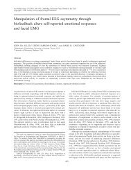
Introduction to Principal Components Analysis of Event-Related
To appear in:
Potentials
Joseph Dien 13 and Gwen A. Frishkoff 2
1 Department of Psychology, Tulane University
2 Department of Psychology, University of Oregon
3 Department of Psychology, University of Kansas
Event Related Potentials: A Methods Handbook. Handy, T. (editor).
Cambridge, Mass: MIT Press.
Address for correspondence: Joseph Dien, Department of Psychology,
426 Fraser Hall, University of Kansas, 1415 Jayhawk Blvd., Lawrence,
KS 66045-7556. E-mail: jdien@ku.edu.
1

Introduction
Over the last several decades, a variety of methods have
been developed for statistical decomposition of event-related
potentials (ERPs). The simplest and most widely applied of these
techniques is principal components analysis (PCA). It belongs to
a class of factor-analytic procedures, which use eigenvalue
decomposition to extract linear combinations of variables
(latent factors) in such a way as to account for patterns of
covariance in the data parsimoniously, that is, with the fewest
factors.
In ERP data, the variables are the microvolt readings
either at consecutive time points (temporal PCA) or at each
electrode (spatial PCA). The major source of covariance is
assumed to be the ERP components, characteristic features of the
waveform that are spread across multiple time points and
multiple electrodes (Donchin & Coles, 1991). Ideally, each
latent factor corresponds to a separate ERP component, providing
a statistical decomposition of the brain electrical patterns
that are superposed in the scalp-recorded data.
PCA has a range of applications for ERP analysis. First, it
can be used for data reduction and cleaning or filtering, prior
2

to data analysis. By reducing hundreds of variables to a handful
of latent factors, PCA can greatly simplify analysis and
description of complex data. Moreover, the factors retained for
further analysis are considered more likely to represent pure
signal (i.e., brain activity), as opposed to noise (i.e.,
artifacts or background EEG).
Second, PCA can be used in data exploration as a way to
detect and summarize features that might otherwise escape visual
inspection. This is particularly useful when ERPs are measured
over many tens or hundreds of recording sites; spatial patterns
can then be used to constrain the decomposition into latent
temporal patterns, as described in the following section.
The use of such high-density ERPs (recordings at 50 or more
electrodes) has become increasingly popular in the last several
years. A striking feature of high-density ERPs is that the
complexity of the data seems to grow exponentially as the number
of recording sites is doubled or tripled. Thus, while increases
in spatial resolution can lead to important new discoveries,
subtle patterns are likely to be missed, as higher spatial
sampling reveals more and more complex patterns, overlapping in
both time and space. A rational approach to data decomposition
can improve the chances of detecting these subtler effects.
3

Third, PCA can serve as an effective means of data
description. In principle, PCA can describe features of the
dataset more objectively and more precisely than is possible
with the unaided eye. Such increased precision could be
especially helpful when PCA is used as a preprocessing step for
ERP source localization (Dien, 1999; Dien, Frishkoff, Cerbonne,
& Tucker, 2003a; Dien, Spencer, & Donchin, 2003b; Dien, Tucker,
Potts, & Hartry, 1997).
Despite the many useful functions of PCA, this method has
had a somewhat checkered history in ERP research, beginning in
the 1960s (Donchin, 1966; Ruchkin, Villegas, & John, 1964). An
influential review paper by Donchin & Heffley (1979) promoted
the use of PCA for ERP component analysis. A few years later,
however, PCA entered something of a dark age in the ERP field
with the publication of a methodological critique (Wood &
McCarthy, 1984), which demonstrated that PCA solutions may be
subject to misallocation of variance across the latent factors.
Wood and McCarthy noted that the same problems arise in the use
of other techniques, such as reaction time and peak amplitude
measures. The difference is that misallocation is made more
explicit in PCA, which they argued should be regarded as an
advantage. Yet this last point was often overlooked, and this
seminal paper has, ironically, been cited as an argument against
4

the use of PCA. Perhaps as a consequence, many researchers
continued to rely on conventional ERP analysis techniques.
More recently, the emergence of high-density ERPs has
revived the interest in PCA as a method of data reduction.
Moreover, some recent studies have shown that statistical
decomposition can lead to novel insights into well-known ERP
effects, providing evidence to help separate ERP components
associated with different perceptual and cognitive operations
(Dien et al., 2003a; Dien, Frishkoff, & Tucker, 2000; Dien et
al., 1997; Spencer, Dien, & Donchin, 2001).
The present review presents a systematic outline of the steps
in temporal PCA, and the issues that arise at each step in
implementation. Some problems and limitations of temporal PCA
are discussed, including rotational indeterminacy, problems of
misallocation, and latency jitter. We then compare some recent
alternatives to temporal PCA, namely: spatial PCA (Dien, 1998a),
sequential (spatio-temporal or temporo-spatial) PCA (Spencer et
al., 2001), parametric PCA (Dien et al., 2003a), multi-mode PCA
(Möcks, 1988), and partial least squares (PLS) (Lobaugh, West, &
McIntosh, 2001). Each technique has evolved to address certain
weaknesses with the traditional PCA method. We conclude with
questions for further research, and advocate a research program
5

for systematic comparison of the strengths and limitations of
different multivariate techniques in ERP research.
Steps in Temporal PCA
The two most common types of factor analysis are principal
axis factors and principal components analysis. These methods
are equivalent for all practical purposes when there are many
variables and when the variables are highly correlated (Gorsuch,
1983), as in most ERP datasets. In the ERP literature PCA is
the more common method. Normally, one and the same term,
"component," has been used for both PCA linear combinations and
for characteristic spatial and temporal features of the ERP. To
avoid confusion, the term factor (or latent factor) will be used
here to refer to PCA (latent) components, and the term component
will be reserved for spatiotemporal features of the ERP
waveform.
The PCA process consists of three main steps: computation
of the relationship matrix, extraction and retention of the
factors, and rotation to simple structure. In the following
sections, PCA simulation is performed to illustrate each step,
using the PCA Toolkit (version 1.06), a set of Matlab functions
for performing PCA on ERP data. This toolkit was written by the
first author and is freely available upon request.
6

The Data Matrix
A key to understanding PCA procedures as applied to ERPs is
to be clear about how multiple sources of variance contribute to
the data decomposition. In temporal PCA, the dataset is
organized with the variables corresponding to time points, and
observations corresponding to the different waveforms in the
dataset, as shown in Figure 1.
Figure 1. Data matrix, with dimensions 20 x 6. Variables are
time points, measured in two conditions for ten subjects. Part
b presents the covariance matrix computed from the data matrix.
7

The waveforms vary across subjects, electrodes, and experimental
conditions. Thus, subject, spatial, and task variance are
collectively responsible for covariance among the temporal
variables. Although it may seem odd to commingle these three
sources of variance, they provide equally valid bases for
distinguishing an ERP component; in this respect, is reasonable
to treat them collectively. For example, the voltage readings
tend to rise and fall together between 250 and 350 ms in a
simple oddball experiment, because they are mutually influenced
by the P300 which occurs during this period. Since individual
differences, scalp location, and experimental task may all
affect the recorded P300 amplitude, the amplitudes of these time
points will likewise covary as a function of these three sources
of variance. Figure 2 shows the grand-averaged waveforms (for
n=10 subjects) corresponding to the simulated data in Figure 1.
For simplicity, this example involves only one electrode site,
ten subjects, and two experimental conditions. In subsequent
sections, we will use these simulated data to help illustrate
the steps in implementation of PCA for ERP analysis.
8

Figure 2. Waveforms for grand-averaged data (n=10),
corresponding to data in Figure 1. Graph displays two non-
overlapping correlated components, plotted for two hypothetical
conditions, A and B.
The Relationship Matrix
The first step in applying PCA is to generate a
relationship (or association) matrix, which captures the
interrelationships between temporal variables. The simplest
such matrix is the sum-of-squares cross-products (SSCP) matrix.
For each pair of variables, the two values for each observation
are multiplied and then added together. Thus, variables that
tend to rise and fall together will produce the highest values
in the matrix. The diagonal of the matrix (the relationship of
each variable to itself) is the sum of the squared values of
each variable. For an example of the effect of using the SSCP
9

matrix, see (Curry, Cooper, McCallum, Pocock, Papakostopoulos,
Skidmore, & Newton, 1983). SSCP treats mean differences in the
same fashion as differences in variance, which has odd effects
on the PCA computations. For example, factors computed on an
SSCP matrix can be correlated, even when they are orthogonal
when using other matrices. In general, we do not recommend the
use of the SSCP matrix in ERP analyses.
An alternative to the SSCP matrix is the covariance matrix.
This matrix is computed in the same fashion as the SSCP matrix,
except that the mean of each variable is subtracted out before
generating the relationship matrix. Mean correction ensures that
variables with high mean values do not have a disproportionate
effect on the factor solution. The effect of mean correction on
the solution depends on the EEG reference site, a topic that is
beyond the scope of this review (cf. Dien, 1998a).
A third alternative is to use the correlation matrix as the
relationship matrix. The correlation matrix is computed in the
same fashion as the covariance matrix, except that the variable
variances are standardized. This is accomplished by first mean
correcting each variable, and then dividing each variable by its
standard deviation, which ensures that the variables contribute
equally to the factor solution. Since time points that do not
10

contain ERP components have smaller variances, this procedure
may exacerbate the influence of background noise. Simulation
studies indicate that covariance matrices can yield more
accurate results (Dien, Beal, & Berg, submitted). We therefore
recommend the use of covariance matrices.
In Figure 3(a), the simulated data are converted into a
covariance matrix. Observe how the time points containing the
two components (t2 and t5) result in larger entries than those
without. The entries with the largest numbers will have the
most influence on the next step in the PCA procedure: factor
extraction.
Factor Extraction
In the extraction stage, a process called eigenvalue
decomposition is performed, which progressively removes linear
combinations of variables that account for the greatest variance
at each step. Each linear combination constitutes a latent
factor. In Figure 3, we demonstrate how this process
iteratively reduces the remaining values in the relationship
matrix to zero.
11

Figure 3. (a) Original covariance matrix. (b) Covariance matrix
after subtraction of Factor 1 (Varimax-rotated; see next
Section). (c) Covariance matrix after subtraction of Factors 1
and 2. Since Factors 1 and 2 together account for nearly all of
the variance, the result is the null matrix.
In general, PCA should extract as many factors as there are
variables, as long as the number of observations is equal to or
12

greater than the number of variables (i.e., as long as the data
matrix is of full rank).
The initial extraction yields an unrotated solution,
consisting of a factor loading matrix and a factor score matrix.
The factor loading matrix represents correlations between the
variables and the factor scores. The factor score matrix
indexes the magnitude of the factors for each of the
observations and thus represents the relationship between the
factors and the observations. If the two matrices are
multiplied together, they will reproduce the data matrix. By
convention, the reproduced data matrix will be in standardized
form, regardless of the type of relationship matrix that was
entered into the PCA. To recreate the original data matrix, the
variables of this standardized matrix are multiplied by the
original standard deviations, and the original variable means
are restored.
13

Figure 4. Reconstructed waveforms, calculated by multiplying the
Factor Loadings by the Factor Scores, scaled to microvolts
(i.e., multiplied by the matrix of standard deviations for the
original data). Data reconstructed using Varimax-rotated factors
for this example.
For a temporal PCA, the loadings describe the time course
of each of the factors. To accurately represent the time course
of the factors, it is necessary to first multiply them by the
variable standard deviations, which rescales them to microvolts
14

(see proof in Dien, 1998a). Further, it is important to note
that the sign of a given factor loading is arbitrary. This is
necessarily the case since a given peak in the factor time
course will be positive on one side of the head, and negative on
the other side, due to the dipolar nature of electrical fields
(Nunez, 1981). Note, further, that the dipolar distributions can
be distorted or obscured by referencing biases in the data
(Dien, 1998b). Only the product of the factor loading and the
factor score corresponds to the original data in an unequivocal
way. Thus, if the factor loading is positive at the peak, then
the factor scores from one side of the head will be positive and
the other side will be negative, corresponding to the dipolar
field.
The factor scores, on the other hand, provide information
about the other sources of variance (i.e., subject, task, and
spatial variance). For example, to compute the amplitude of a
factor at a specific electrode site for a given task condition,
one simply takes the factor scores corresponding to the
observations for that task at the electrode of interest and
computes their mean (across subjects). If this mean value is
computed for each electrode, the resulting values can be used to
plot the scalp topography for that factor. If a specific time
point is chosen, it is possible reconstruct the scalp topography
15

with the proper microvolt scaling by multiplying the mean scores
by the factor loading and the standard deviation for the time
point of interest (see proof in Dien, 1998a).
Unlike the PCA algorithm in most statistics packages, the
PCA Toolkit does not mean-correct the factor scores. This
maintains an interpretable relationship between the factor
scores and the original data. If factor scores are mean-
corrected as part of the standardization, the mean task scores
will be centered around zero, which can make factor
interpretation more difficult. In an oddball experiment, for
example, the P300 factor scores should be large for the target
condition and small for the standard condition. However, if the
factor scores are mean-corrected, then the mean task scores for
the two conditions will be of equal amplitude and opposite signs
(since mean correction splits the difference).
Factor Retention
Most of the PCA factors that are extracted account for
small proportions of variance, which may be attributed to
background noise, or minor departures from group trends. In the
interest of parsimony, only the larger factors are typically
retained, since they are considered most likely to contain
interpretable signal. A common criterion for determining how
16

many factors to retain is the scree test (Cattell, 1966; Cattell
& Jaspers, 1967). This test is based on the principle that the
PCA of a random set of data will produce a set of randomly sized
factors. Since factors are extracted in order of descending
size, when their sizes are graphed they will form a steady
downward slope. A dataset containing signal, in addition to the
noise, should have initial factors that are larger than would be
expected from random data alone. The point of departure from
the slope (the elbow) indicates the number of factors to retain.
Factors beyond this point are likely to contain noise and are
best dropped. Figure 5 plots the reconstructed grand-averaged
data, using the retained factors in order to verify that
meaningful factors have not been excluded.
17

Figure 5. Reconstructed waveforms, computed as in Figure 4,
using only Factors 1 and 2. Because the first two factors
account for nearly all of the variance, the reconstruction is
nearly as good as the original data (cf. Fig. 2).
In practice, the scree plot for ERP datasets often contains
multiple elbows, which can make it difficult to determine the
proper number of factors to retain. Part of the problem is that
the noise contains some unwanted signal (remnants of the
background EEG). A modified version of the parallel test can be
used to address this issue (Dien, 1998a). The parallel test
determines how many factors represent signal by comparing the
scree produced by the full dataset to that produced when only
the noise is present. The noise level is estimated by
generating an ERP average with every other trial inverted, which
has the effect of canceling out the signal while leaving the
noise level unchanged. The results of the parallel test should
be considered a lower bound since retaining additional factors
to account for major noise features can actually improve the
analysis (for such an exampole, see Dien, 1998a), although in
principle if too many additional factors are retained it can
result in unwanted distinctions being made (such as between
subject-specific variations of the component). In general, the
experience of the first author is that between eight and sixteen
18

factors is often appropriate, although this may depend, among
other things, on the number of recording sites.
Factor Rotation
A critical step, after deciding how many factors to retain,
is to determine the best way of allocating variance across the
remaining factors. Unfortunately, there is no transparent
relationship between the PCA factors and the latent variables of
interest (i.e., ERP components). Eigenvalue decomposition
blindly generates factors that account for maximum variance,
which may be influenced by more than one latent variable;
whereas, the goal is to have each factor represent a single ERP
component.
As shown in Figure 6, there is not a one-to-one mapping of
factors to variables after the initial factor extraction.
Rather, the initial extraction has maximized the variance of the
first factor by including variance from as many variables as
possible. In doing so, it has generated a factor that is a
hybrid of two ERP components, the linear sum of roughly 10% of
the P1 and 90% of the P3. The second factor contains the
leftover variance of both components. This example demonstrates
the danger of interpreting the initial unrotated factors
19

directly, as is sometimes advocated (e.g., Rösler & Manzey,
1981).
Figure 6. Graph of unrotated factors. Only Factors 1 and 2
are graphed, since Factors 3–6 are close to 0.
Factor rotation is used to restructure the allocation of
variables to factors to maximize the chance that each factor
reflects a single latent variable. The most common rotation is
Varimax (Kaiser, 1958). In Varimax, each of the retained
factors is iteratively rotated pairwise with each of the other
factors in turn, until changes in the solution become
negligible. More specifically, the Varimax procedure rotates the
20

two factors such that the sum of the factor loadings (raised to
the fourth power) is maximized. This has the effect of favoring
solutions in which factor loadings are as extreme as possible
with a combination of near-zero loadings and large peak values.
Since ERP components (other than DC potentials) tend to have
zero activity for most of the epoch with a single major peak or
dip, Varimax should yield a reasonable approximation to the
underlying ERP components (Fig. 7). Temporal overlap of ERP
components raises additional issues, which are addressed in the
following section.
21

Figure 7. Graph of Varimax-rotated Factor Loadings. Only Factors
1 and 2 are graphed, since Factors 3–6 are close to 0.
Simulation studies have demonstrated that the accuracy of a
rotation is influenced by several situations, including
component overlap and component correlation (Dien, 1998a).
Component overlap is a problem, because the more similar two ERP
components are, the more difficult it is to distinguish them
(Möcks & Verleger, 1991). Further, correlations between
components may lead to violations of statistical assumptions.
The initial extraction and the subsequent Varimax rotation
maintain strict orthogonality between the factors (so the
factors are uncorrelated). To the extent that the components
are in fact correlated, the model solution will be inaccurate,
producing misallocation of variance across the factors.
Component correlation can arise when two components respond to
the same task variables (an example is the P300 and Slow Wave
components, which often co-occur), or when both components
respond to the same subject parameters (e.g., age, sex, or
personality traits), or share a common spatial distribution.
Further, these two components can be measured at some of the
same electrodes due to their similar scalp topographies.
22

Component correlation can be effectively addressed by using
an oblique rotation, such as Promax (Hendrickson & White, 1964),
allowing for correlated factors (Dien, 1998a). In Promax, the
initial Varimax rotation is succeeded by a "relaxation" step, in
which each individual factor is further rotated to maximize the
number of variables with minimal loadings. A factor is adjusted
in this fashion without regard to the other factors, allowing
factors to become correlated, and thus relaxing the
orthogonality constraint in the Varimax solution. The Promax
rotation typically leads to solutions that more accurately
capture the large features of the Varimax factors while
minimizing the smaller features. As a result, Promax solutions
tend to account for slightly less variance than the original
Varimax solutions, but may also give more accurate results
(Dien, 1998a). A typical result can be seen in Figure 8.
23

Figure 8. Graph of Promax-rotated Factor Loadings. Only Factors
1 and 2 are graphed, since Factors 3–6 are close to 0.
Spatial versus Temporal PCA
A limitation of temporal PCA is that factors are defined
solely as a function of component time course, as instantiated
by the factor loadings. This means that ERP components which
are topographically distinct, but have a similar time course,
will be modeled by a single factor. A sign that this has
occurred is when temporal PCA yields condition effects
characterized by a scalp topography that differs from the
overall factor topography.
24

To address this problem, spatial PCA may be used as an
alternative to temporal PCA (Dien, 1998a). In a spatial PCA,
the data are arranged such that the variables are electrode
locations, and observations are experimental conditions,
subjects, and time points. The factor loadings therefore
describe scalp topographies, instead of temporal patterns. This
approach is less likely to confound ERP components with the same
time course. as long as they are differentiated by the task or
subject variance. On the other hand, it will be subject to the
converse problem, confusing components with similar scalp
topographies, even when they have clearly separate time
dynamics.
The choice between spatial versus temporal PCA should
depend on specific analysis goals. A rule of thumb is that if
time course is the focus of an analysis, then spatial PCA should
be used, and vice versa. The reason is that the factor loadings
are constrained to be the same across the entire dataset (i.e.,
the same time course for temporal PCA, and the same scalp
topography for spatial PCA). The factor scores, on the other
hand, are free to vary between conditions and subjects. Thus,
one can examine latency changes with spatial, but not temporal,
PCA, and vice versa. In particular, this implies that temporal,
25

ather than spatial, PCA should be more effective as a
preprocessing step in source localization, since these modeling
procedures rely on the scalp topography to infer the number and
configuration of sources.
All other things being equal, temporal PCA is in principle
more accurate than spatial PCA, since component overlap reduces
PCA accuracy, and volume conduction ensures that all ERP
components will overlap in a spatial PCA. Furthermore, the
effect of the Varimax and Promax rotations is to minimize factor
overlap, which is a more appropriate goal for temporal than for
spatial PCA. A caveat in either case is that ERP component
separation can be achieved only if subject or task variance (or
both) can effectively distinguish the components. In other
words, the three sources of variance associated with each
observation must collectively be able to distinguish the ERP
components, regardless of whether the components differ along
the variable dimension (time for temporal PCA, or space for
spatial PCA).
Recent alternatives to PCA
In recent years, a variety of multivariate statistical
techniques have been developed and are increasingly making their
way into the ERP literature. One such method, independent
26

components analysis (Makeig, Bell, Jung, & Sejnowski, 1996), is
discussed elsewhere in this volume.
In this section, we present four multivariate techniques in
ERP analysis, which share a common basis in their use of
eigenvalue decomposition. Each technique has been claimed to
address one or more problems with conventional PCA. The
application these techniques in ERP research is very recent, and
more work is needed to characterize their respective strengths
and limitations for various ERP applications. Future
developments of these techniques may lead to a powerful suite of
tools that can be used to address a range of problems in ERP
analysis.
Sequential spatiotemporal (or temporospatial) PCA
A recent procedure for improved separation of ERP
components is spatiotemporal (or temporospatial) PCA (Spencer,
Dien, & Donchin, 1999; Spencer et al., 2001). In this
procedure, ERP components that were confounded in the initial
PCA are separated by the application of a second PCA, which is
used to separate variance along the other dimension. For a
temporospatial PCA this is accomplished by rearranging the
factor scores resulting from the temporal PCA so that each
column contains the factor scores from a different electrode. A
27

spatial PCA can then be conducted using these factor scores as
the new variables. While the temporal variance has been
collapsed by the initial PCA, the subject and task variance are
still expressed in the observations, and can thus be used to
separate ERP components that were confounded in the initial PCA.
In Spencer, et al. (1999, 2001), the initial spatial PCA
was followed by a temporal PCA, with the factor scores from all
the factors combined within the same analysis (number of
observations equal to number of subjects x number of tasks x
number of spatial factors). This procedure led to a clear
separation of the P300 from the Novelty P3. However, it also had
an important drawback: the application of a single temporal PCA
to all the spatial factors could result in loss of some of the
finer distinctions in time course between different spatial
factors. This analytic strategy was necessary because the
generalized inverse function, used by SAS to generate the factor
scores, requires that there be more observations than variables.
The PCA Toolkit has bypassed this requirement by directly
rotating the factor scores (Möcks & Verleger, 1991), allowing
each initial factor to be subjected to a separate PCA (following
the example of Scott Makeig’s ICA toolbox and an independent
suggestion by Bill Dunlap). In a more recent study (Dien et al.,
28

2003b), an initial spatial PCA yielded 12 factors; each spatial
factor was then subjected to a separate temporal PCA (each
retaining four factors for simplicity's sake). For analyses
using this newer approach (it makes little difference for the
original approach), temporospatial PCA is recommended over
spatiotemporal PCA, since temporal PCA may lead to better
initial separation of ERP components. Subsequent application of
a spatial PCA can then help separate components that were
confounded in the temporal PCA. On the other hand, if latency
analysis is a goal of the PCA, then spatial PCA should be done
first (since latency analysis cannot be done on the results of a
temporal PCA) with the succeeding temporal PCA step used to
verify whether multiple components are present in the factor of
interest, as demonstrated in another recent study (Dien,
Spencer, & Donchin, in press).
The full equation to generate the microvolt value for a
specific time point t and channel c for a spatiotemporal PCA is
L1 * V1 * L2 * S2 * V2 (where L1 is the spatial PCA factor
loading for c, V1 is the standard deviation of c, L2 is the
temporal PCA factor loading for t, S2 is the mean factor scores
for the temporal factor, and V2 is the standard deviation of the
spatial factor scores at t. The temporal and spatial terms are
reversed for temporospatial PCA.
29

Parametric PCA
Another recent method involves the use of parametric
measures to improve PCA separation of latent factors, which
differ along one or more stimulus dimension (Dien et al.,
2003a). This more specialized procedure can only be conducted
on datasets containing observations with a continuous range of
values. In Dien, et al. (2003), ERP responses to sentence
endings were averaged for each stimulus item (collapsing over
subjects) rather than averaging over subjects (collapsing over
items in each experimental condition). This item-averaging
approach resulted in 120 sentence averages, which were rated on
a number of linguistic parameters, such as meaningfulness and
word frequency. After an initial temporal PCA, it was then
possible to correlate the parameter of interest with the mean
factor score at each channel, to determine the influence of the
stimulus parameter on a given ERP component, such as the N400.
This had the effect of highlighting the relationship between ERP
components and stimulus parameters, while factoring out the
effects of ERP components unrelated to the parameters of
interest. In this fashion, parametric PCA can lead to scalp
topographies that reflect only the parameters of interest,
providing a new approach to functional separation of ERP
components. This approach thus provides an alternative method to
30

sequential PCA for deconfounding components. These components
can be then be subjected to further analyses, such as dipole and
linear inverse modeling.
Partial Least Squares
Partial least squares (PLS), like PCA, is a multivariate
technique based on eigenvalue decomposition. Unlike PCA, PLS
operates on the covariance between the data matrix and a matrix
of contrasts that represents features of the experimental design
(McIntosh, Bookstein, Haxby, & Grady, 1996). Similar to
parametric PCA procedures, the decomposition is focused on
variance due to the experimental manipulations (condition
differences). A recent paper (Lobaugh et al., 2001) applied PLS
to ERP data for the first time. Simulations showed that the PLS
analysis led to accurate modeling of the spatial and temporal
effects that were associated with condition differences in the
ERP waveforms. Lobaugh, et al., also suggest that PLS may be an
effective preprocessing method, identifying time points and
electrodes that are sensitive to condition differences and can
therefore be targeted for further analyses.
One cautionary note concerning PLS arises from the use of
difference waves, which are created by subtracting the ERP
waveform in one experimental condition from the response in a
31

different condition, in order to isolate experimental effects
prior to factor extraction. This approach, based on the logic of
subtraction, can lead to incorrect conclusions when the
assumption of pure insertion is violated, that is, when two
conditions are different in kind rather than in degree. It can
also produce misleading results when a change in latency appears
to be an amplitude effect or when multiple effects appear to be
a single effect.
Neuroimaging measures, such as ERP and fMRI, may be
particularly subject to such misinterpretations, since both
spatial (anatomical) and temporal, variance can lead to
condition differences. If these multiple sources of variance not
adequately separated, a temporal difference between conditions
may be erroneously ascribed to a single anatomical region or ERP
component (e.g., (Zarahn, Aguirre, & D'Esposito, 1999). In a
recent example (Spencer, Abad, & Donchin, 2000), PCA was used to
examine the claim that recollection (as compared with
familiarity) is associated with a unique electrophysiological
component. Spencer, et al., concluded that the effect was more
accurately ascribed to differences in latency jitter, or trial-
to-trial variance in peak latency of the P300 across the two
conditions.
32

For this reason, condition differences, while useful,
should only be interpreted in respect to the overall patterns in
the original data. Further, both spatial and temporal variance
between conditions should be analyzed fully, to rule out
differences in latency jitter or other electrophysiological
effects that may be hidden or confounded through cognitive
subtraction. This recommendation also applies to the
interpretation of results from the use of partial variance
techniques, such as PLS.
Multi-Mode Factor Analysis
The techniques discussed in previous sections were all
based on two-mode (defined as a dimension of variance) analysis
of ERP data. In temporal PCA, for instance, time points
represent one dimension (variables axis), and the other
dimension combines the remaining sources of variance — i.e.,
subjects, electrodes, and experimental conditions (observations
axis). By contrast, multi-mode procedures analyze the data
across three or more dimensions simultaneously. For example, in
trilinear decomposition (TLD), the subject data matrix X i is
expressed as the cross-product of three factors, as shown in
equation (1):
X i =B *A i *C, (1)
33

where B is a set of spatial components and C is a set of
temporal components. A i represents the subject loadings on B and
C. B and C are calculated in separate, spatial and temporal,
singular value decompositions of the data and are then combined
to yield a new decomposition of the data, for any fixed
dimensionality (Wang, Begleiter, & Porjesz, 2000). Since tri-
mode PCA is susceptible to the same rotational indeterminacies
as regular PCA, rotational procedures will need to be developed
and evaluated.
It has been claimed that tri-mode PCA can effectively remove
“nuisance” sources of variance, as described by Möcks (1985),
providing greater sensitivity as compared with conventional,
two-dimensional PCA. Further, Achim has described the use of
multi-modal procedures to help address misallocation of variance
(Achim & Bouchard, 1997). These reports point to the need for
thorough and systematic comparison of multi-mode methods such as
TLD with other methods, such as parametric PCA and PLS. This
can only be done for algorithms that are made available to the
rest of the research community, either through open source or
through commercial software packages.
34

Conclusion
PCA and related procedures can provide an effective way to
preprocess high-density ERP datasets, and to help separate
components that differ in their sensitivity to spatial,
temporal, or functional parameters. This brief review has
attempted to characterize the current state of the art in PCA of
ERPs. Ongoing research will continue to refine and optimize
statistical procedures and will aim to determine the optimal
procedures for statistical decompositions of ERP data.
Ultimately, it is likely that a range of statistical tools will
be required, each best suited to different applications in ERP
analysis.
35

Bibliography
Achim, A., & Bouchard, S. (1997). Toward a dynamic topographic
components model. Electroencephalography and Clinical
Neurophysiology, 103, 381-385.
Cattell, R. B. (1966). The scree test for the number of factors.
Multivariate Behavioral Research, 1, 245-276.
Cattell, R. B., & Jaspers, J. (1967). A general plasmode (No.
3010-5-2) for factor analytic exercises and research.
Multivariate Behavioral Research Monographs, 67-3, 1-212.
Curry, S. H., Cooper, R., McCallum, W. C., Pocock, P. V.,
Papakostopoulos, D., Skidmore, S., et al. (1983). The
principal components of auditory target detection. In A. W.
K. Gaillard & W. Ritter (Eds.), Tutorials in ERP research:
Endogenous components (pp. 79-117). Amsterdam: North-
Holland Publishing Company.
Dien, J. (1998a). Addressing misallocation of variance in
principal components analysis of event-related potentials.
Brain Topography, 11(1), 43-55.
36

Dien, J. (1998b). Issues in the application of the average
reference: Review, critiques, and recommendations.
Behavioral Research Methods, Instruments, and Computers,
30(1), 34-43.
Dien, J. (1999). Differential lateralization of trait anxiety
and trait fearfulness: evoked potential correlates.
Personality and Individual Differences, 26(1), 333-356.
Dien, J., Beal, D., & Berg, P. (submitted). Optimizing principal
components analysis for event-related potential analysis.
Dien, J., Frishkoff, G. A., Cerbonne, A., & Tucker, D. M.
(2003a). Parametric analysis of event-related potentials in
semantic comprehension: Evidence for parallel brain
mechanisms. Cognitive Brain Research, 15, 137-153.
Dien, J., Frishkoff, G. A., & Tucker, D. M. (2000).
Differentiating the N3 and N4 electrophysiological semantic
incongruity effects. Brain & Cognition, 43, 148-152.
Dien, J., Spencer, K. M., & Donchin, E. (2003b). Localization of
the event-related potential novelty response as defined by
principal components analysis. Cognitive Brain Research,
17, 637-650.
Dien, J., Spencer, K. M., & Donchin, E. (in press). Parsing the
"Late Positive Complex": Mental chronometry and the ERP
37

components that inhabit the neighborhood of the P300.
Psychophysiology.
Dien, J., Tucker, D. M., Potts, G., & Hartry, A. (1997).
Localization of auditory evoked potentials related to
selective intermodal attention. Journal of Cognitive
Neuroscience, 9(6), 799-823.
Donchin, E. (1966). A multivariate approach to the analysis of
average evoked potentials. IEEE Transactions on Bio-Medical
Engineering, BME-13, 131-139.
Donchin, E., & Coles, M. G. H. (1991). While an undergraduate
waits. Neuropsychologia, 29(6), 557-569.
Donchin, E., & Heffley, E. (1979). Multivariate analysis of
event-related potential data: A tutorial review. In D. Otto
(Ed.), Multidisciplinary perspectives in event-related
potential research (EPA 600/9-77-043) (pp. 555-572).
Washington, DC: U.S. Government Printing Office.
Gorsuch, R. L. (1983). Factor analysis (2nd ed.). Hillsdale, NJ:
Lawrence Erlbaum Associates.
Hendrickson, A. E., & White, P. O. (1964). Promax: A quick
method for rotation to oblique simple structure. The
British Journal of Statistical Psychology, 17, 65-70.
38

Kaiser, H. F. (1958). The varimax criterion for analytic
rotation in factor analysis. Psychometrika, 23, 187-200.
Lobaugh, N. J., West, R., & McIntosh, A. R. (2001).
Spatiotemporal analysis of experimental differences in
event-related potential data with partial least squares.
Psychophysiology, 38(3), 517-530.
Makeig, S., Bell, A. J., Jung, T., & Sejnowski, T. J. (1996).
Independent component analysis of electroencephalographic
data. Advances in Neural Information Processing Systems, 8,
145-151.
McIntosh, A. R., Bookstein, F. L., Haxby, J. V., & Grady, C. L.
(1996). Spatial pattern analysis of functional brain images
using Partial Least Squares. Neuroimage, 3, 143-157.
Möcks, J. (1988). Topographic components model for event-related
potentials and some biophysical considerations. IEEE
Transactions on Biomedical Engineering, 35(6), 482-484.
Möcks, J., & Verleger, R. (1991). Multivariate methods in
biosignal analysis: application of principal component
analysis to event-related potentials. In R. Weitkunat
(Ed.), Digital Biosignal Processing (pp. 399-458).
Amsterdam: Elsevier.
39

Nunez, P. L. (1981). Electric fields of the brain: The
neurophysics of EEG. New York: Oxford University Press.
Rösler, F., & Manzey, D. (1981). Principal components and
varimax-rotated components in event-related potential
research: Some remarks on their interpretation. Biological
Psychology, 13, 3-26.
Ruchkin, D. S., Villegas, J., & John, E. R. (1964). An analysis
of average evoked potentials making use of least mean
square techniques. Annals of the New York Academy of
Sciences, 115(2), 799-826.
Spencer, K. M., Abad, E. V., & Donchin, E. (2000). On the search
for the neurophysiological manifestation of recollective
experience. Psychophysiology, 37, 494-506.
Spencer, K. M., Dien, J., & Donchin, E. (1999). A componential
analysis of the ERP elicited by novel events using a dense
electrode array. Psychophysiology, 36, 409-414.
Spencer, K. M., Dien, J., & Donchin, E. (2001). Spatiotemporal
Analysis of the Late ERP Responses to Deviant Stimuli.
Psychophysiology, 38(2), 343-358.
Wang, K., Begleiter, H., & Porjesz, B. (2000). Trilinear
modeling of event-related potentials. Brain Topography,
12(4), 263-271.
40

Wood, C. C., & McCarthy, G. (1984). Principal component analysis
of event-related potentials: Simulation studies demonstrate
misallocation of variance across components.
Electroencephalography and Clinical Neurophysiology, 59,
249-260.
Zarahn, E., Aguirre, G. K., & D'Esposito, M. (1999). Temporal
isolation of the neural correlates of spatial mnemonic
processing with fMRI. Cognitive Brain Research, 7(3), 255-
268.
41