Apostol T.M. Modular..
Apostol T.M. Modular..
Apostol T.M. Modular..

Create successful ePaper yourself
Turn your PDF publications into a flip-book with our unique Google optimized e-Paper software.
Graduate Texts in Mathematics 41<br />
Editorial Board<br />
J.H. Ewing F.W. Gehring P.R. Halmos
Graduate Texts in Mathematics<br />
l TAKEUTIIZARING. Introduction to Axiomatic Set Theory. 2nd ed.<br />
2 OXTOBY. Measure and Category. 2nd ed.<br />
3 ScHAEFFER. Topological Vector Spaces.<br />
4 HILTON/STAMMBACH. A Course in Homological Algebra.<br />
5 MAc LANE. Categories for the Working Mathematician.<br />
6 HUGHES/PiPER. Projective Planes.<br />
7 SERRE. A Course in Arithmetic.<br />
8 T AKEUTIIZARING. Axiomatic Set Theory.<br />
9 HUMPHREYS. Introduction to Lie Algebras and Representation Theory.<br />
10 COHEN. A Course in Simple Homotopy Theory.<br />
ll CoNWAY. Functions of One Complex Variable. 2nd ed.<br />
12 BEALS. Advanced Mathematical Analysis.<br />
l3 ANDERSON/FULLER. Rings and Categories of Modules.<br />
14 GOLUBITSKY/GUILLEMIN. Stable Mappings and Their Singularities.<br />
15 BERBERIAN. Lectures in Functional Analysis and Operator Theory.<br />
16 WINTER. The Structure of Fields.<br />
17 RosENBLATT. Random Processes. 2nd ed.<br />
18 HALMOS. Measure Theory.<br />
19 HALMOS. A Hilbert Space Problem Book. 2nd ed., revised.<br />
20 HUSEMOLLER. Fibre Bundles. 2nd ed.<br />
21 HUMPHREYS. Linear Algebraic Groups.<br />
22 BARNEs/MACK. An Algebraic Introduction to Mathematical Logic.<br />
23 GREUB. Linear Algebra. 4th ed.<br />
24 HoLMES. Geometric Functional Analysis and its Applications.<br />
25 HEWITT/STROMBERG. Real and Abstract Analysis.<br />
26 MANES. Algebraic Theories.<br />
27 KELLEY. General Topology.<br />
28 ZARISKIISAMUEL. Commutative Algebra. Vol. I.<br />
29 ZARISKIISAMUEL. Commutative Algebra. Vol. II.<br />
30 JACOBSON. Lectures in Abstract Algebra 1: Basic Concepts.<br />
31 JACOBSON. Lectures in Abstract Algebra II: Linear Algebra.<br />
32 JACOBSON. Lectures in Abstract Algebra III: Theory of Fields and Galois Theory.<br />
33 HIRSCH. Differential Topology.<br />
34 SPITZER. Principles of Random Walk. 2nd ed.<br />
35 WERMER. Banach Algebras and Several Complex Variables. 2nd ed.<br />
36 KELLEYINAMIOKA et al. Linear Topological Spaces.<br />
37 MONK. Mathematical Logic.<br />
38 GRAUERT/FRITZSCHE. Several Complex Variables.<br />
39 ARVESON. An Invitation to C*-Algebras.<br />
40 KEMENY/SNELL/KNAPP. Denumerable Markov Chains. 2nd ed.<br />
41 APOSTOL. <strong>Modular</strong> Functions and Dirichlet Series in Number Theory. 2nd ed.<br />
42 SERRE. Linear Representations of Finite Groups.<br />
43 GILLMAN/JERISON. Rings of Continuous Functions.<br />
44 KENDIG. Elementary Algebraic Geometry.<br />
45 LoE.vE. Probability Theory I. 4th ed.<br />
46 LoEVE. Probability Theory II. 4th ed.<br />
47 MoiSE. Geometric Topology in Dimensions 2 and 3.<br />
contmuttd after lndel
Tom M. <strong>Apostol</strong><br />
<strong>Modular</strong> Functions<br />
and Dirichlet Series<br />
in Number Theory<br />
Second Edition<br />
With 25 Illustrations<br />
Springer-Verlag<br />
New York Berlin Heidelberg<br />
London Paris Tokyo Hong Kong
Tom M. <strong>Apostol</strong><br />
Department of Mathematics<br />
California Institute of Technology<br />
Pasadena, CA 91125<br />
USA<br />
Editorial Board<br />
J.H. Ewing<br />
Department of<br />
Mathematics<br />
Indiana University<br />
Bloomington, IN 47405<br />
USA<br />
F. W. Gehring<br />
Department of<br />
Mathematics<br />
University of Michigan<br />
Ann Arbor, MI 48109<br />
USA<br />
AMS Subject Classifications<br />
IOA20, 10A45, IOD45, 10H05, !OHIO, 10120, 30Al6<br />
P.R. Halmos<br />
Department of<br />
Mathematics<br />
Santa Clara University<br />
Santa Clara, CA 95053<br />
USA<br />
Library of Congress Cataloging-in-Publication Data<br />
<strong>Apostol</strong>, Tom M.<br />
<strong>Modular</strong> functions and Dirichlet series in number theory/Tom M. <strong>Apostol</strong>.-2nd ed.<br />
p. cm.-(Graduate texts in mathematics; 41)<br />
Includes bibliographical references.<br />
ISBN 0-387-97127-0 (alk. paper)<br />
I. Number theory. 2. Functions, Elliptic. 3. Functions, <strong>Modular</strong>. 4. Series,<br />
Dirichlet. I. Title. II. Series.<br />
QA241.A62 1990<br />
512'.7---dc20 89-21760<br />
Printed on acid-free paper.<br />
© 1976, 1990 Springer-Verlag New York, Inc.<br />
All rights reserved. This work may not be translated or copied in whole or in part without the<br />
written permission of the publisher (Springer-Verlag New York, Inc., 17::l Fifth Avenue, New<br />
York, NY 10010, USA), except for brief excerpts in connection with reviews or scholarly<br />
analysis. Use in connection with any form of information and retrieval, electronic adaptation,<br />
computer software, or by similar or dissimilar methodology now known or hereafter developed<br />
is forbidden.<br />
The use of general descriptive names, trade names, trademarks. etc., in this publication, even if<br />
the former are not especially identified, is not to be taken as a sign that such names, as<br />
understood by the Trade Marks and Merchandise Marks Act, may accordingly be used freely<br />
by anyone.<br />
Typeset by Asco Trade Typesetting Ltd., Hong Kong.<br />
Printed and bound by Edwards Brothers, Inc., Ann Arbor, Michigan.<br />
Printed in the United States of America.<br />
9 8 7 6 5 4 3 2 I<br />
ISBN 0-387-97127-0 Springer-Verlag New York Berlin Heidelberg<br />
ISBN 3-540-97127-0 Springer-Verlag Berlin Heidelberg New York
Preface<br />
This is the second volume of a 2-volume textbook* which evolved from a<br />
course (Mathematics 160) offered at the California Institute of Technology<br />
during the last 25 years.<br />
The second volume presupposes a background in number theory comparable<br />
to that provided in the first volume, together with a knowledge of<br />
the basic concepts of complex analysis.<br />
Most of the present volume is devoted to elliptic functions and modular<br />
functions with some of their number-theoretic applications. Among the<br />
major topics treated are Rademacher's convergent series for the partition<br />
function, Lehner's congruences for the Fourier coefficients of the modular<br />
functionj('r), and Heeke's theory of entire forms with multiplicative Fourier<br />
coefficients. The last chapter gives an account of Bohr's theory of equivalence<br />
of general Dirichlet series.<br />
Both volumes of this work emphasize classical aspects of a subject which<br />
in recent years has undergone a great deal of modern development. It is<br />
hoped that these volumes will help the nonspecialist become acquainted<br />
with an important and fascinating part of mathematics and, at the same<br />
time, will provide some of the background that belongs to the repertory of<br />
every specialist in the field.<br />
This volume, like the first, is dedicated to the students who have taken<br />
this course and have gone on to make notable contributions to number<br />
theory and other parts of mathematics.<br />
T.M.A.<br />
January, 1976<br />
*The first volume is in the Springer-Verlag series Undergraduate Texts in Mathematics under<br />
the title Introduction to Analytic Number Theory.<br />
v
Preface to the Second Edition<br />
The major change is an alternate treatment of the transformation formula for<br />
the Dedekind eta function, which appears in a five-page supplement to Chapter<br />
3, inserted at the end of the book (just before the Bibliography). Otherwise,<br />
the second edition is almost identical to the first. Misprints have been<br />
repaired, there are minor changes in the Exercises, and the Bibliography has<br />
been updated.<br />
T.M.A.<br />
July, 1989
Chapter 1<br />
Elliptic functions<br />
1.1 Introduction<br />
1.2 Doubly periodic functions<br />
1.3 Fundamental pairs of periods<br />
1.4 Elliptic functions<br />
1.5 Construction of elliptic functions<br />
1.6 The Weierstrass p function<br />
1. 7 The Laurent expansion of p near the origin<br />
1.8 Differential equation satisfied by f.J<br />
1.9 The Eisenstein series and the invariants 9 2 and 9 3<br />
1.10 The numbers e1 , e2 , e3<br />
1.11 The discriminant A<br />
1.12 Klein's modular function J(r)<br />
1.13 Invariance of J under unimodular transformations<br />
1.14 The Fourier expansions of 9z(r) and 9 3(-r:)<br />
1.15 The Fourier expansions of A(r) and J(r)<br />
Exercises for Chapter 1<br />
Chapter 2<br />
The <strong>Modular</strong> group and modular functions<br />
2.1 Mobius transformations<br />
2.2 The modular group r<br />
2.3 Fundamental regions<br />
2.4 <strong>Modular</strong> functions<br />
Contents<br />
1<br />
1<br />
2<br />
4<br />
6<br />
9<br />
11<br />
11<br />
12<br />
13<br />
14<br />
15<br />
16<br />
18<br />
20<br />
23<br />
26<br />
28<br />
30<br />
34<br />
vii
2.5 Special values of J 39<br />
2.6 <strong>Modular</strong> functions as rational functions of J 40<br />
2. 7 Mapping properties of J 40<br />
2.8 Application to the inversion problem for Eisenstein series 42<br />
2.9 Application to Picard's theorem 43<br />
Exercises for Chapter 2 44<br />
Chapter 3<br />
The Dedekind eta function<br />
3.1 Introduction 47<br />
3.2 Siegel's proof of Theorem 3.1 48<br />
3.3 Infinite product representation for Ll( r) 50<br />
3.4 The general functional equation for ry(r) 51<br />
3.5 Iseki's transformation formula 53<br />
3.6 Deduction of Dedekind's functional equation from Iseki's<br />
formula 58<br />
3.7 Properties of Dedekind sums 61<br />
3.8 The reciprocity law for Dedekind sums 62<br />
3.9 Congruence properties of Dedekind sums 64<br />
3.10 The Eisenstein series G2(r) 69<br />
Exercises for Chapter 3 70<br />
Chapter 4<br />
Congruences for the coefficients of the modular function j<br />
4.1 Introduction 74<br />
4.2 The subgroup r 0(q) 75<br />
4.3 Fundamental region of r 0 (p) 76<br />
4.4 Functions automorphic under the subgroup r 0(p) 78<br />
4.5 Construction of functions belonging tor 0(p) 80<br />
4.6 The behavior of fP under the generators of r 83<br />
4.7 The function
5.5 Ford circles<br />
5.6 Rademacher's path of integration<br />
5. 7 Rademacher's convergent series for p(n)<br />
Exercises for Chapter 5<br />
Chapter 6<br />
<strong>Modular</strong> forms with multiplicative coefficients<br />
99<br />
102<br />
104<br />
110<br />
6.1 Introduction 113<br />
6.2 <strong>Modular</strong> forms of weight k 114<br />
6.3 The weight formula for zeros of an entire modular form 115<br />
6.4 Representation of entire forms in terms of G 4 and G 6 117<br />
6.5 The linear space Mk and the subspace Mk, 0 118<br />
6.6 Classification of entire forms in terms of their zeros 119<br />
6. 7 The Heeke operators Tn 120<br />
6.8 Transformations of order n 122<br />
6.9 Behavior of Tnfunder the modular group 125<br />
6.10 Multiplicative property of Heeke operators 126<br />
6.11 Eigenfunctions of Heeke operators 129<br />
6.12 Properties of simultaneous eigenforms 130<br />
6.13 Examples of normalized simultaneous eigenforms 131<br />
6.14 Remarks on existence of simultaneous eigenforms in M lk, 0 133<br />
6.15 Estimates for the Fourier coefficients of entire forms 134<br />
6.16 <strong>Modular</strong> forms and Dirichlet series 136<br />
Exercises for Chapter 6 138<br />
Chapter 7<br />
Kronecker's theorem with applications<br />
7.1 Approximating real numbers by rational numbers 142<br />
7.2 Dirichlet's approximation theorem 143<br />
7.3 Liouville's approximation theorem 146<br />
7.4 Kronecker's approximation theorem: the one-dimensional<br />
case 148<br />
7.5 Extension of Kronecker's theorem to simultaneous<br />
approximation 149<br />
7.6 Applications to the Riemann zeta function 155<br />
7.7 Applications to periodic functions 157<br />
Exercises for Chapter 7 159<br />
Chapter 8<br />
General Dirichlet series and Bohr's equivalence theorem<br />
8.1 Introduction 161<br />
8.2 The half-plane of convergence of general Dirichlet series 161<br />
8.3 Bases for the sequence of exponents of a Dirichlet series 166<br />
IX
8.4 Bohr matrices 167<br />
8.5 The Bohr function associated with a Dirichlet series 168<br />
8.6 The set of values taken by a Dirichlet seriesf(s) on a line<br />
u = u0<br />
8. 7 Equivalence of general Dirichlet series 173<br />
8.8 Equivalence of ordinary Dirichlet series 174<br />
8.9 Equality of the sets UtCu 0 ) and Ug(u 0 ) for equivalent<br />
Dirichlet series 176<br />
8.10 The set of values taken by a Dirichlet series in a neighborhood<br />
of the line u = u0<br />
8.11 Bohr's equivalence theorem 178<br />
8.12 Proof of Theorem 8.15 179<br />
8. 13 Examples of equivalent Dirichlet series. Applications of Bohr's<br />
theorem to £-series 184<br />
8.14 Applications of Bohr's theorem to the Riemann zeta function 184<br />
Exercises for Chapter 8 187<br />
Supplement to Chapter 3 190<br />
Bibliography 196<br />
Index of special symbols 199<br />
Index 201<br />
X<br />
170<br />
176
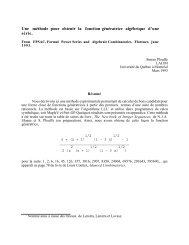
1.3: Fundamental pairs of periods<br />
(a) (b)<br />
Figure 1.1<br />
Theorem 1.1. If (wb w 2) is a fundamental pair of periods, then the triangle<br />
with vertices 0, Wt. w 2 contains no further periods in its interior or on its<br />
boundary. Conversely, any pair of periods with this property is fundamental.<br />
PROOF. Consider the parallelogram with vertices 0, wb w1 + w 2, and w 2,<br />
shown in Figure 1.2a. The points inside or on the boundary of this parallelogram<br />
have the form<br />
z = aw 1 + f3w 2 ,<br />
where 0 ::s;; a ::s;; 1 and 0 ::s;; f3 ::s;; 1. Among these points the only periods are 0,<br />
w1 , w 2, and w1 + w 2, so the triangle with vertices 0, w1 , w 2 contains no<br />
periods other than the vertices.<br />
0 0<br />
(a) (b)<br />
Figure 1.2<br />
3
1.4: Elliptic functions<br />
Constant functions are trivial examples of elliptic functions. Later we<br />
shall give examples ofnonconstant elliptic functions, but first we derive some<br />
fundamental properties common to all elliptic functions.<br />
Theorem 1.3. A nonconstant elliptic function has afundamental pair of periods.<br />
PROOF. Iffis elliptic the set of points wherefis analytic is an open connected<br />
set. Also, f has two periods with nonreal ratio. Among all the nonzero<br />
periods off there is at least one whose distance from the origin is minimal<br />
(otherwisefwould have arbitrarily small nonzero periods and hence would<br />
be constant). Let w be one of the nonzero periods nearest the origin. Among<br />
all the periods with modulus I w I choose the one with smallest nonnegative<br />
argument and call it w 1 . (Again, such a period must exist otherwise there<br />
would be arbitrarily small nonzero periods.) If there are other periods<br />
with modulus I w 1 I besides w 1 and - w 1, choose the one with smallest<br />
argument greater than that of w1 and call this w 2 • If not, find the next<br />
larger circle containing periods # nw1 and choose that one of smallest<br />
nonnegative argument. Such a period exists since f has two noncollinear<br />
periods. Calling this one w 2 we have, by construction, no periods in the<br />
triangle 0, wl> w 2 other than the vertices, hence the pair (w 1, w 2} is fundamental.<br />
D<br />
Iff and g are elliptic functions with periods w 1 and w2 then their sum,<br />
difference, product and quotient are also elliptic with the same periods. So,<br />
too, is the derivativef'.<br />
Because of periodicity, it suffices to study the behavior of an elliptic<br />
function in any period parallelogram.<br />
Theorem 1.4. /fan ellipticfunctionfhas no poles in some period parallelogram,<br />
thenfis constant.<br />
PROOF. Iffhas no poles in a period parallelogram, thenfis continuous and<br />
hence bounded on the closure of the parallelogram. By periodicity, f is<br />
bounded in the whole plane. Hence, by Liouville's theorem,fis constant. D<br />
Theorem 1.5. If an elliptic functionfhas no zeros in some period parallelogram,<br />
thenfis constant.<br />
PROOF. Apply Theorem 1.4 to the reciprocal 1/f D<br />
Note. Sometimes it is inconvenient to have zeros or poles on the boundary<br />
of a period parallelogram. Since a meromorphic function has only a<br />
finite number of zeros or poles in any bounded portion of the plane, a period<br />
parallelogram can always be translated to a congruent parallelogram with<br />
no zeros or poles on its boundary. Such a translated parallelogram, with no<br />
zeros or poles on its boundary, will be called a cell. Its vertices need not be<br />
periods.<br />
5
1 : Elliptic functions<br />
Theorem 1.6. The contour integral of an elliptic function taken along the<br />
boundary of any cell is zero.<br />
PROOF. The integrals along parallel edges cancel because of periodicity. D<br />
Theorem 1.7. The sum of the residues of an elliptic function at its poles in any<br />
period parallelogram is zero.<br />
PROOF. Apply Cauchy's residue theorem to a cell and use Theorem 1.6. D<br />
\<br />
Note. Theorem 1. 7 shows that an elliptic function which is not constant<br />
has at least two simple poles or at least one double pole in each period<br />
parallelogram.<br />
Theorem 1.8. The number of zeros of an elliptic function in any period parallelogram<br />
is equal to the number of poles, each counted with multiplicity.<br />
PROOF. The integral<br />
_1 J f'(z) dz<br />
2ni c f(z) '<br />
taken around the boundary C of a cell, counts the difference between the<br />
number of zeros and the number of poles insid'e the cell. But f'lf is elliptic<br />
with the same periods asf, and Theorem 1.6 tells us that this integral is zero.<br />
D<br />
Note. The number of zeros (or poles) of an elliptic function in any period<br />
parallelogram is called the order of the function. Every nonconstant elliptic<br />
function has order ;;;:: 2.<br />
1.5 Construction of elliptic functions<br />
We turn now to the problem of constructing a nonconstant elliptic function.<br />
We prescribe the periods and try to find the simplest elliptic function having<br />
these periods. Since the order of such a function is at least 2 we need a<br />
second order pole or two simple poles in each period parallelogram. The<br />
two possibilities lead to two theories of elliptic functions, one developed by<br />
Weierstrass, the other by Jacobi. We shall follow Weierstrass, whose point<br />
of departure is the construction of an elliptic function with a pole of order<br />
2 at z = 0 and hence at every period. Near each period w the principal part<br />
of the Laurent expansion must have the form<br />
6<br />
A B<br />
z-w z-w<br />
( )<br />
2 +--.
and<br />
1.10: The numbers e 1, e2 , e3<br />
n-2<br />
(2n + 3)(n - 2)b(n) = 3 L b(k)b(n - 1 - k) for n ::2: 3,<br />
k=l<br />
or equivalently,<br />
m-2<br />
(2m+ l)(m- 3)(2m- l)G2m = 3 L (2r - 1)(2m- 2r- l)G2rG2m-2r<br />
r=2<br />
form ::2:4.<br />
PROOF. Differentiation of the differential equation for f.J gives another<br />
differential equation of second order satisfied by f.J,<br />
(5)<br />
Now we write f.J(z) = z- 2 + L:'= 1 b(n)z 2 " and equate like powers of z<br />
in (5) to obtain the required recursion relations. D<br />
Definition. We denote by e1, e2 , e3 the values of f.J at the half-periods,<br />
The next theorem shows that these numbers are the roots of the cubic<br />
polynomial4g;J 3 - 92f.J - 93·<br />
Theorem 1.14. We have<br />
4g;J 3(z) - 92 f.J(z) - 93 = 4(f.J(z) - e1)(f.J(z) - e2)(f.J(z) - e3).<br />
Moreover, the roots e1, e2 , e3 are distinct, hence g2 3 - 27g/ # 0.<br />
PROOF. Since f.J is even, the derivative f.J' is odd. But it is easy to show that<br />
the half-periods of an odd elliptic function are either zeros or poles. In fact,<br />
by periodicity we have f.J'( -!w) = f.J'(w - !w) = f.J'(!w), and since f.J' is odd<br />
we also have f.J'( -!w) = - f.J'(!w). Hence f.J'(!w) = 0 if f.J'(!w) is finite.<br />
Since f.J'(z) has no poles at !w1 , !w2 , !(w1 + w2 ), these points must be<br />
zeros of f.J'. But f.J' is of order 3, so these must be simple zeros of f.J'. Thus<br />
f.J' can have no further zeros in the period-parallelogram with vertices<br />
0, w 1, w2 , w 1 + w2 . The differential equation shows that each of these points<br />
is also a zero of the cubic, so we have the factorization indicated.<br />
Next we show that the numbers e 1, e2 , e3 are distinct. The elliptic function<br />
f.J(z)- e1 vanishes at z = !w1. This is a double zero since f.J'(!w 1) = 0.<br />
Similarly, f.J(z)- e2 has a double zero at !w2. If e1 were equal to e2, the<br />
elliptic function f.J(z) - e1 would have a double zero at !w1 and also a double<br />
13
2 The<br />
modular group<br />
and modular functions<br />
2.1 Mobius transformations<br />
In the foregoing chapter we encountered unimodular transformations<br />
, ar + b<br />
r=-er<br />
+ d<br />
where a, b, e, d are integers with ad - be = 1. This chapter studies such<br />
transformations in greater detail and also studies functions which, like<br />
J(r), are invariant under unimodular transformations. We begin with some<br />
remarks concerning the more general transformations<br />
(1)<br />
f(z) = az + b<br />
ez + d<br />
where a, b, e, d are arbitrary complex numbers.<br />
Equation (1) definesf(z) for all z in the extended complex number system<br />
C* = C u { oo} except for z = -d/e and z = oo. We extend the definition<br />
off to all of C* by defining<br />
and<br />
with the usual convention that z/0 = oo if z :f. 0.<br />
First we note that<br />
(2)<br />
a<br />
f(oo) = -,<br />
e<br />
f(w) _ f(z) = (ad - be)(w - z)<br />
(ew + d)(ez + d)'<br />
which shows thatfis constant if ad - be = 0. To avoid this degenerate case<br />
we assume that ad - be :f. 0. The resulting rational function is called a<br />
26
(1)<br />
p<br />
/<br />
"'<br />
/<br />
/<br />
__ ..... ooi __<br />
Figure 2.3<br />
.... ,<br />
' '<br />
(4)<br />
p + 1<br />
2.4: <strong>Modular</strong> functions<br />
PROOF. Assume first that f has no zeros or poles on the finite part of the<br />
boundary of Rr· Cut Rr by a horizontal line, Im('r) = M, where M > 0 is<br />
taken so large that all the zeros or poles off are inside the truncated region<br />
which we call R. [Iff had an infinite number of poles in Rr they would have<br />
an accumulation point at ioo, contradicting condition (c). Similarly, since f<br />
is not identically zero, f cannot have an infinite number of zeros in Rr.]<br />
Let oR denote the boundary of the truncated region R. (See Figure 2.4.)<br />
Let N and P denote the number of zeros and poles off inside R. Then<br />
1 {1 l l l l }<br />
N - P = - 1 i f'(7:) - d1: = - + + + +<br />
2ni oR j(1:) 2ni (1) (Zl (J) (5)<br />
where the path is split into five parts as indicated in Figure 2.5. The integrals<br />
along (1) and (4) cancel because of periodicity. They also cancel along (2)<br />
and (3) because (2) gets mapped onto (3) with a reversal of direction under<br />
-t + -<br />
iM ..------------, t + iM<br />
-<br />
R t<br />
p p + 1<br />
Figure 2.4<br />
35
2: The modular group and modular functions<br />
PROOF. We assume f is an entire function which omits two values, say a<br />
and b, a i= b, and show thatfis constant. Let<br />
( ) _ f(z)- a<br />
g z - b .<br />
-a<br />
Then g is entire and omits the values 0 and 1.<br />
The upper half-plane H is covered by the images of the closure of the<br />
fundamental region Rr under transformations of r. Since J maps the closure<br />
of Rr onto the complex plane, J maps the half-plane H onto an infinitesheeted<br />
Riemann surface with branch points over the points 0, 1 and oo<br />
(the images of the vertices p, i and oo, respectively). The inverse function J- 1<br />
maps the Riemann surface back onto the closure of the fundamental region<br />
Rr. Since J'(r) i= 0 if r i= p orr i= i and since J'(p) = J'(i) = 0, each singlevalued<br />
branch of J- 1 is locally analytic everywhere except at 0 = J(p ),<br />
1 = J(i), and oo = J( oo ). For each single-valued branch of r 1 the composite<br />
function<br />
h(z) = r 1[g(z)]<br />
is a single-valued function element which is locally analytic at each finite<br />
z since g(z) is never 0 or 1. Therefore his arbitrarily continuable in the entire<br />
finite z-plane. By the monodromy theorem, the continuation of h exists as a<br />
single-valued function analytic in the entire finite z-plane. Thus his an entire<br />
function and so too is<br />
But Im h(z) > 0 since h(z) E H so<br />
cp(z) = eih(z).<br />
jcp(z)j = e-Imh(z) < 1.<br />
Therefore cp is a bounded entire function which, by Liouville's theorem,<br />
must be constant. But this implies h is constant and hence g is constant since<br />
g(z) = J[h(z)]. Thereforefis constant sincef(z) =a + (b - a)g(z). D<br />
Exercises for Chapter 2<br />
In these exercises, r denotes the modular group, S and T denote its generators,<br />
S(r) = -1/r, T(r) = r + 1, and I denotes the identity element.<br />
1. Find all elements A of r which (a) commute with S; (b) commute with ST.<br />
2. Find the smallest integer n > 0 such that (ST)" = I.<br />
3. Determine the point r in the fundamental region Rr which is equivalent to<br />
(a) (8 + 6i)/(3 + 2i); (b) (!Oi + ll)/(6i + 12).<br />
4. Determine all elements A of r which leave i fixed.<br />
44<br />
5. Determine all elements A of r which leave p = e 2 nil 3 fixed.
3.1 Introduction<br />
The Dedekind eta function<br />
3<br />
In many applications of elliptic modular functions to number theory the<br />
eta function plays a central role. It was introduced by Dedekind in 1877<br />
and is defined in the half-plane H = {r: Im(r) > 0} by the equation<br />
(1)<br />
rJ(r) = e"it/12 fl (1 _ e2"inr).<br />
n=1<br />
The infinite product has the form fl (1 - x") where x = e2"ir. If r E H then<br />
I xI < 1 so the product converges absolutely and is nonzero. Moreover,<br />
since the convergence is uniform on compact subsets of H, rJ(r) is analytic<br />
on H.<br />
The eta function is closely related to the discriminant Ll(r) introduced<br />
in Chapter 1. Later in this chapter we show that<br />
00<br />
Ll(r) = (2n) 12 rJ 24(r).<br />
This result and other properties of rJ(r) follow from transformation formulas<br />
which describe the behavior of rJ(r) under elements of the modular group r.<br />
For the generator Tr = r + 1 we have<br />
00<br />
(2) rJ(r + 1) = e"i(t+ 1)/12 fl (1 _ e2"in(t+ 1)) = e"i/12rJ(r).<br />
n=1<br />
Consequently, for any integer b we have<br />
(3) rJ(T +b)= e"ib/12rJ(T).<br />
Equation (2) also shows that rJ24(r) is periodic with period 1.<br />
47
4 Congruences<br />
4.1 Introduction<br />
for the coefficients<br />
of the modular function}<br />
The function j(r) = 12 3 J(r) has a Fourier expansion of the form<br />
1 00 .<br />
j(r) = - + L c(n)xn, (x = e 2m)<br />
X n=O<br />
where the coefficients c(n) are integers. At the end of Chapter 1 we mentioned<br />
a number of congruences involving these integers. This chapter shows how<br />
some of these congruences are obtained. Specifically we will prove that<br />
c(2n)=O (mod2 11 ),<br />
c(3n) = 0 (mod 3 5 ),<br />
c(5n) = 0 (mod 5 2 ),<br />
c(7n) = 0 (mod 7).<br />
The method used to obtain these congruences can be illustrated for the<br />
modulus 5 2 . We consider the function<br />
00<br />
/ 5(r) = I c(5n)xn<br />
n=l<br />
obtained by extracting every fifth coefficient in the Fourier expansion of j.<br />
Then we show that there is an identity of the form<br />
(1)<br />
where the a; are integers and
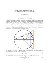
-1<br />
I<br />
-2<br />
I<br />
0<br />
Figure 4.1 Fundamental region for r 0(3)<br />
4.3: Fundamental region of r 0(p)<br />
Next we prove (ii). Suppose r 1 E R, r 2 E R and Vr 1 = r 2 for some V in<br />
r 0(p). We will prove that r 1 = r 2 • There are three cases to consider:<br />
(a) r 1 ERr, r 2 ERr. In this case r 1 = r 2 since VEr.<br />
(b) r 1 ERr, r 2 E STk(Rr).<br />
(c) r 1 E STk'(Rr), r 2 E STk 2(Rr).<br />
In case (b), r 2 = STkr3 where r 3 ERr. The equation<br />
implies<br />
v = STk = G<br />
This contradicts the fact that v E r o(p).<br />
Finally, consider case (c). In this case<br />
and<br />
-1)<br />
where r 1' and r 2 ' are in Rr. Since Vr 1 = r 2 we have VSTk'r1 ' = STk 2r/ so<br />
VSTk' = STk 2 ,<br />
k .<br />
I<br />
2<br />
T<br />
77
4: Congruences for the coefficients of the modular function j<br />
Since VEr0(p) this requires k 2 = k 1 (modp). But both k 1 , k 2 are in the<br />
interval [0, p- 1], so k2 = k 1• Therefore<br />
v = ST 0 S = S 2 = 1<br />
and r 1 = r 2 . This completes the proof. 0<br />
We mention (without prooO the following theorem of Rademacher [34]<br />
concerning the generators of r 0(p). (This theorem is not needed in the<br />
later work.)<br />
Theorem 4.3. For any prime p > 3 the subgroup r 0(p) has 2[pj12] + 3<br />
generators and they may be selected from the following elements:<br />
where Tr = r + 1, Sr = -1/r, and<br />
k'<br />
V. = STkST-k'S = (<br />
k -(kk' + 1)<br />
where kk' = - 1 (mod p), The subgroup r 0 (2) has generators T and V1;<br />
the subgroup r 0(3) has generators T and V2 ,<br />
Here is a short table of generators:<br />
p 2 3 5 7 11 13 17 19<br />
Generators: T T T T T T T T<br />
vl v2 v2 v3 v4 v4 v4 Vs<br />
v3 Vs v6 Vs v7 Vs<br />
Vs v9 v12<br />
v!O v13 v!3<br />
4.4 Functions automorphic ur1der the<br />
subgroup r o(p)<br />
We recall that a modular function f is one which has the following three<br />
properties:<br />
(a) f is meromorphic in the upper half-plane H,<br />
(b) f(Ar) = f(r) for every transformation A in the modular group r,<br />
(c) The Fourier expansion off has the form<br />
78<br />
00<br />
f(rl = I ane2ttinr,<br />
n= -m
If property (b) is replaced by<br />
4.4: Functions automorphic under the subgroup r 0(p)<br />
(b') f(Vr) = f(r) for every transformation V in r 0(p),<br />
thenfis said to be automorphic under the subgroup r 0(p). We also say that<br />
f belongs to r o(p).<br />
The next theorem shows that the only bounded functions belonging to<br />
r 0(p) are constants.<br />
Theorem 4.4. Iff is automorphic under r 0(p) and bounded in H, then f is<br />
constant.<br />
PROOF. According to Theorem 4.1, for every v in r there exists an element<br />
Pin r 0(p) and an integer k, 0 :::; k :::; p, such that<br />
V = PAk><br />
where Ak = STk if k < p, and AP = I. For each k = 0, 1, ... , p, let<br />
rk = {PAk:PEro(p)}.<br />
Each set rk is called a right coset of r 0(p). Choose an element J1k from the<br />
coset rk and define a function fk on H by the equation<br />
fk(r) = f(l-k r).<br />
Note that fp(r) = f(Pr) = f(r) since P E r 0(p) and f is automorphic under<br />
r 0(p). The function value fk(r) does not depend on which element J1k was<br />
chosen from the coset r k because<br />
fk(r) = f(J!k r) = f(PAk r) = f(Ak r)<br />
and the element Ak is the same for all members of the coset r k.<br />
How does fk behave under the transformations of the full modular group?<br />
If V E r then<br />
fk(Vr) = f(l-k Vr).<br />
Now J1k VErso there is an element Q in r 0(p) and an integer m, 0 :::; m :::; p,<br />
such that<br />
Therefore we have<br />
Moreover, as k runs through the integers 0, 1, 2, ... , p so does m. In other<br />
words, there is a permutation a of {0, 1, 2, ... , p} such that<br />
fk(Vr) = fa(kl(r) for each k = 0, 1, ... , p.<br />
Now choose a fixed win Hand let<br />
p<br />
q>(r) = n {fk(r) - f(w)}.<br />
k;Q<br />
79
4: Congruences for the coefficients of the modular function j<br />
2. Let G denote the subgroup of r generated by the transformations Sand T 2 , where<br />
Sr = -1/r and Tr = T + 1.<br />
(a) If(: :) E G prove that a = d (mod 2) and b = c (mod 2).<br />
(b) If V E G prove that there exist elements A and B of r such that<br />
Vr 2 + 1 =A(': 1) and Vr + 1 = B(r + 1).<br />
(c) If (: :) E G and c > 0 prove that<br />
( aT+ b) 9 cr + d = e(a, b, c, d){- i(cr + dW 129(r), where I e(a, b, c, d) I = 1. Express e(a, b, c, d) in terms of Dedekind sums.<br />
Exercises 3 through 8 outline a proof(due to Mordell [28]) of the multiplicativity<br />
of Ramanujan's function
5 Rademacher's<br />
5.1 Introduction<br />
series for<br />
the partition function<br />
The unrestricted partition function p(n) counts the number of ways a positive<br />
integer n can be expressed as a sum of positive integers ::::;; n. The number of<br />
summands is unrestricted, repetition is allowed, and the order of the summands<br />
is not taken into account.<br />
The partition function is generated by Euler's infinite product<br />
(1)<br />
where p(O) = 1. Both the product and series converge absolutely and represent<br />
the analytic function Fin the unit disk I xI < 1. A proof of (1) and other<br />
elementary properties of p(n) can be found in Chapter 14 of [ 4]. This chapter<br />
is concerned with the behavior of p(n) for large n.<br />
The partition function p(n) satisfies the asymptotic relation<br />
eK,Jii<br />
p(n) "' ;; as n -+ oo,<br />
4ny3<br />
where K = n:(2/3) 1 i 2 . This was first discovered by Hardy and Ramanujan [13]<br />
in 1918 and, independently, by J. V. Uspensky [52] in 1920. Hardy and<br />
Ramanujan proved more. They obtained a remarkable asymptotic formula<br />
of the form<br />
(2) p(n) = L Pk(n) " + O(n- 114 ),<br />
k
Equation (9) also yields the following theorem.<br />
5.5: Ford circles<br />
Theorem 5.4. Given 0 :s;; ajb < cjd :s;; 1 with be - ad = 1, let h/k be the<br />
mediant of ajb and cjd. Then a/b < h/k < cjd, and these fractions satisfy<br />
the unimodular relations<br />
bh- ak = 1, ck- dh = 1.<br />
PROOF. Since h/k lies between ajb and cjd we have bh- ak 2 1 and<br />
ck - dh 2 1. Equation (9) shows that k = b + d if, and only if, bh - ak =<br />
ck- dh = 1. D<br />
The foregoing theorems tell us how to construct F n + 1 from F n.<br />
Theorem 5.5. The set F n + 1 includes F n. Each fraction in F n + 1 which is not in<br />
Fn is the mediant of a pair of consecutive fractions in Fn. Moreover, if<br />
ajb < cjd are consecutive in any Fn, then they satisfy the unimodular<br />
relation be - ad = 1.<br />
PROOF. We use induction on n. When n = 1 the fractions 0/1 and 1/1 are<br />
consecutive and satisfy the unimodular relation. We pass from F 1 to F 2 by<br />
inserting the mediant 1/2. Now suppose a/b and cjd are consecutive in F"<br />
and satisfy the unimodular relation be - ad = 1. By Theorem 5.3, they will<br />
be consecutive in F m for all m satisfying<br />
max(b, d) :s;; m :s;; b + d - 1.<br />
Form their mediant h/k, where h = a + c, k = b + d. By Theorem 5.4<br />
we have bh - ak = 1 and ck - dh = 1 so h and k are relatively prime.<br />
The fractions ajb and cjd are consecutive in F m for all m satisfying<br />
max(b, d) :s;; m :s;; b + d- 1, but are not consecutive in Fk since k = b + d<br />
and h/k lies in Fk between ajb and cjd. But the two new pairs a/b < h/k and<br />
h/k < c/darenowconsecutiveinFkbecausek = max(b,k)andk = max(d,k).<br />
The new consecutive pairs still satisfy the unimodular relations bh - ak = 1<br />
and ck - dh = 1. This shows that in passing from F n to F" + 1 every new<br />
fraction inserted must be the mediant of a consecutive pair in F "'and the new<br />
consecutive pairs satisfy the unimodular relations. Therefore F n+ 1 has these<br />
properties ifF" does. D<br />
5.5 Ford circles<br />
Definition. Given a rational number h/k with (h, k) = 1. The Ford circle<br />
belonging to this fraction is denoted by C(h,· k) and is that circle in the<br />
complex plane with radius 1/(2k 2 ) and center at the point (h/k) + i/(2k 2 )<br />
(see Figure 5.1).<br />
Ford circles are named after L. R. Ford [9] who first studied their<br />
properties in 1938.<br />
99
5: Rademacher's series for the partition function<br />
h<br />
k<br />
Figure 5.1 The Ford circle C(h, k)<br />
Theorem 5.6. Two Ford circles C(a, b) and C(c, d) are either tangent to each<br />
other or they do not intersect. They are tangent if, and only if, be - ad =<br />
± 1. In particular, Ford circles of consecutive Farey fractions are tangent<br />
to each other.<br />
PROOF. The square of the distance D between centers is (see Figure 5.2)<br />
a<br />
b<br />
Figure 5.2<br />
whereas the square of the sum of their radii is<br />
( 1 1 )2<br />
c<br />
d<br />
(r + R)2 = 2b2 + 2d2 .<br />
The difference D 2 - (r + R) 2 is equal to<br />
Moreover, equality holds if, and only if (ad - bc) 2 = 1.<br />
100<br />
0
5: Rademacher's series for the partition function<br />
To obtain the last statement, it suffices to show that the angle() in Figure<br />
5.3 is n/2. For this it suffices to show that the imaginary part of rt 1(h, k) is<br />
the geometric mean of a and a', where<br />
a = k(k2 + k 1 2)<br />
(See Figure 5.4.) Now<br />
and this completes the proof.<br />
and<br />
' h h1 1<br />
a = - - - - a = - - a.<br />
k k1 kkl<br />
k1 ( k 2 ) 1<br />
= e(k2 + k1 2 ) k1(k 2 + k/) = (k2 + k/) 2 '<br />
Figure 5.4<br />
5.6 Rademacher's path of integration<br />
For each integer N we construct a path P(N) joining the points i and i + 1<br />
as follows. Consider the Ford circles for the Farey series F v· If h1/k 1 < h/k<br />
< h2/k2 are consecutive in FN, the points of tangency of C(/1 1, kd, C(h, k),<br />
and C(h 2 , k2 ) divide C(h, k) into two arcs, an upper arc and a lower arc.<br />
P(N) is the union of the upper arcs so obtained. For the fractions 0/1 and 1/1<br />
we use only the part of the upper arcs lying above the unit interval [0, 1].<br />
EXAMPLE. Figure 5.5 shows the path P(3).<br />
Because of Theorem 5. 7, the path P(N) always lies above the row of semicircles<br />
connecting adjacent Farey fractions in F N·<br />
The path P(N) is the contour used by Rademacher as a path of integration.<br />
It is convenient at this point to discuss the effect of a certain change of variable<br />
on each circle C(h, k).<br />
Theorem 5.8. The transformation<br />
z = -zk . 2( r- k h)<br />
102<br />
a<br />
D
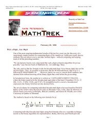
0<br />
I<br />
3<br />
I<br />
2<br />
Figure 5.5 The Rademacher path P(3)<br />
2<br />
3<br />
5.6: Rademacher's path of integration<br />
i +I<br />
maps the Ford circle C(h, k) in the r-plane onto a circle Kin the z-plane of<br />
radius -! about the point z = -! as center (see Figure 5.6). The points of<br />
contact rx1(h, k) and rxih, k) of Theorem 5.7 are mapped onto the points<br />
and<br />
k 2 kk<br />
Zt(h,k) = k2 + k/ + i k2 + lk12<br />
The upper arc joining rx 1(h, k) with rx 2(h, k) maps onto that arc of K which<br />
does not touch the imaginary z-axis.<br />
0<br />
z-plane<br />
Figure 5.6<br />
103
6.4: Representation of entire forms in terms of G4 and G6<br />
6.4 Representation of entire forms in terms<br />
ofG4 and G6<br />
In Chapter 1 it was shown that every Eisenstein series Gk with k > 2 is a<br />
polynomial in G 4 and G 6 . This section shows that the same is true of every<br />
entire modular form. Since the discriminant A is a polynomial in G4 and<br />
G6,<br />
A= g2 3 - 27g 3 2 = (60G4 ) 3 - 27(140G6)2,<br />
it suffices to show that all entire forms of weight k can be expressed in terms<br />
of Eisenstein series and powers of A. The proof repeatedly uses the fact that<br />
the productfg of two entire formsf and g of weights w1 and w2 , respectively,<br />
is another entire form of weight w1 + w2 , and the quotientf/g is an entire<br />
form of weight w1 - w2 if g has no zeros in H or at ioo.<br />
Notation. We denote by Mk the set of all entire modular forms of weight k.<br />
Theorem 6.3. Let f be an entire modular form of even weight k 2:: 0 and define<br />
G0(r) = 1 for all r. Then f can be expressed in one and only one way as a<br />
sum of the type<br />
[k/12)<br />
(7)<br />
f= L a,Gk-12rA',<br />
r=O<br />
k-12r,.2<br />
where the a, are complex numbers. The cusp forms of even weight k are<br />
those sums with a0 = 0.<br />
PRooF. If k < 12 there is at most one term in the sum and the theorem can<br />
be verified directly. Iff has weight k < 12 the weight formula (5) implies<br />
N = N(ioo) = 0 so the only possible zeros off are at the vertices p and i.<br />
For example, if k = 4 we have N(p) = 1 and N(i) = 0. Since G4 has this<br />
property,f/G4 is an entire modular form of weight 0 and therefore is constant,<br />
so f = a0 G4 . Similarly, we find f = a0 Gk if k = 6, 8 or 10. The theorem<br />
also holds trivially for k = 0 (since f is constant) and for k = 2 (since the<br />
sum is empty). Therefore we need only consider even k 2:: 12.<br />
We use induction on k together with the simple observation that every<br />
cusp form in M k can be written as a product Ah, where hEM k-!2.<br />
Assume the theorem has been proved for all entire forms of even weight<br />
6: <strong>Modular</strong> forms with multiplicative coefficients<br />
Dividing each b1 by p 1 - 1 we can write<br />
b, = q,pr-1 + r,,<br />
where 0 ::;; r, < p'- 1 and q, runs through a complete residue system mod p.<br />
Since f is periodic with period 1 we have<br />
( pr-tr: + b,) = (p'-'r: + r,)<br />
f t p 1 f p t-1 '<br />
so as q, runs through a complete residue system mod peach term is repeated<br />
p times. Replacing the index t by t - 1 we see that the last sum is pk- 1 times<br />
the sum defining {T(p'- 1)/}(r:). This proves (29).<br />
Now we consider general powers of the same prime, say m = p• and<br />
n = p'. Without loss of generality we can assume that r ::;; s. We will use induction<br />
on r to prove that<br />
(31)<br />
for all r and all s 2 r. When r = 1, (31) follows for all s 2 1 from (29).<br />
Therefore we assume that (31) holds for r and all smaller powers and all<br />
s 2 r, and prove it also holds for r + 1 and all s 2 r + 1.<br />
By (29) we have<br />
T(p)T(p')T(p•) = T(p'+ 1)T(p") + pk- 1 T(p'- 1)T(p'),<br />
and by the induction hypothesis we have<br />
r<br />
T(p)T(p')T(ps) = L pt(k-1)T(p}T(p'+s-2t).<br />
t=O<br />
Equating the two expressions, solving for T(p'+ 1 )T(p•) and using (29) in the<br />
sum on t we find<br />
r r<br />
T(p'+ 1 )T(p•) = L p'(k-1)T(pr+s+ 1- 21) + L p
7 Kronecker's<br />
theorem<br />
with applications<br />
7.1 Approximating real numbers by rational<br />
numbers<br />
Every irrational number () can be approximated to any desired degree of<br />
accuracy by rational numbers. In fact, if we truncate the decimal expansion<br />
of () after n decimal places we obtain a rational number which differs from<br />
()by less than 10-". However, the truncated decimals might have very large<br />
denominators. For example, if<br />
() = n- 3 = 0.141592653 ...<br />
the first five decimal approximations are 0.1, 0.14, 0.141, 0.1415, 0.14159.<br />
Written in the form a/b, where a and b are relatively prime integers, these<br />
rational approximations become<br />
1 7 141 283 14159<br />
10' 50' 1000' 2000' 100,000"<br />
On the other hand, the fraction 1/7 = 0.142857 ... differs from() by less than<br />
2/1000 and is nearly as good as 141/1000 for approximating(), yet its denominator<br />
7 is very small compared to 1000.<br />
This example suggests the following type of question: Given a real<br />
number (), is there a rational number h/k which is a good approximation to<br />
() but whose denominator k is not too large?<br />
This is, of course, a vague question because the terms "good approximation"<br />
and "not too large" are vague. Before we make the question more<br />
precise we formulate it in a slightly different way. If () - h/k is small, then<br />
(k() - h)/k is small. For this to be small without k being large the numerator<br />
k() - h should be small. Therefore, we can ask the following question:<br />
142
7.2: Dirichlet's approximation theorem<br />
Given a real number() and given e > 0, are there integers hand k such that<br />
lk()- hi< e?<br />
The following theorem of Dirichlet answers this question in the affirmative.<br />
7.2 Dirichlet's approximation theorem<br />
Theorem 7.1. Given any real() and any positive integer N, there exist integers<br />
h and k with 0 < k ::; N such that<br />
(1)<br />
1<br />
lk()- hi< N"<br />
PROOF. Let {x} = x - [x] denote the fractional part of x. Consider the<br />
N + 1 real numbers<br />
0, {()}, {2()}, ... , {N()}.<br />
All these numbers lie in the half open unit interval 0 :s; {m(J} < 1. Now<br />
divide the unit interval into N equal half-open subintervals of length 1/N.<br />
Then some subinterval must contain at least two of these fractional parts,<br />
say {a()} and {b()}, where 0 ::; a < b :s; N. Hence we can write<br />
(2)<br />
But<br />
1<br />
I {b()} - {ae} I < N.<br />
{b()} - {a()} = b() - [b()] - a() + [a()] = (b - a)() - ([b()] - [a()]).<br />
Therefore if we let<br />
inequality (2) becomes<br />
k=b-a<br />
and h = [b()] - [a()]<br />
1<br />
lk()- hi < N' with 0 < k ::; N.<br />
This proves the theorem. 0<br />
Note. Given e > 0 we can choose N > 1/e and (1) implies lk()- hi< e.<br />
The next theorem shows that we can choose h and k to be relatively<br />
prime.<br />
Theorem 7.2. Given any real() and any positive integer N, there exist relatively<br />
prime integers h and k with 0 < k ::; N such that<br />
1<br />
lk()- hi< N"<br />
143
7.5: Extension of Kronecker's theorem to simultaneous approximation<br />
Now choose the largest integer N which satisfies {ke} < 1/N. Then we have<br />
1 1<br />
N + 1 < {ke} < N'<br />
Therefore {mke} = m{ke} form= 1, 2, ... , N, so theN numbers<br />
{ke}, {2ke}, ... , {Nke}<br />
form an increasing equally-spaced chain running from left to right in the<br />
interval (0, 1). The last member of this chain (by the definition of N) satisfies<br />
the inequality<br />
or<br />
N<br />
-- 1 < {Nke} < 1,<br />
N+<br />
1<br />
1 - N + 1 < {Nke} < 1.<br />
Thus {Nke} differs from 1 by less than 1/(N + 1) < {ke} < e. Therefore the<br />
first N members of the subsequence {nke} subdivide the unit interval into<br />
subintervals of length 0, there exist<br />
integers h and k with k > 0 such that<br />
Ike - h - ex I < e.<br />
PROOF. Write ex = [ex] + {ex}. By Theorem 7.7 there exists k > 0 such that<br />
I {ke} - {ex} I < e. Hence<br />
or<br />
lkO- [ke] -(ex- [cx])l < e<br />
Ike- ([ke] - [ex])- cxl
7: Kronecker's theorem with applications<br />
It turns out that this problem cannot always be solved as stated. For example,<br />
suppose we start with two irrational numbers, say 01 and 201, and two real<br />
numbers IX1 and IX 2 , and suppose there exist integers h1, h2 and k such that<br />
and<br />
lk01- h1- IX1I < e<br />
12k(}1 - h2- IX2I ... , cn implies c1 = · · · = cn = 0. This restriction<br />
is compensated for, in part, by removing the restriction that the (}i be<br />
irrational. First we prove what appears to be a less general result.<br />
Theorem 7.9 (First form of Kronecker's theorem). If IX 1, .•• , 1Xn are arbitrary<br />
real numbers, if (}1> •.. , (}n are linearly independent real numbers, and if<br />
e > 0 is arbitrary, then there exists a real number t and integers h1, .•• , hn<br />
such that<br />
I tOi - hi - IXd < e for i = 1, 2, ... , n.<br />
Note. The theorem exhibits a real number t, whereas we asked for an<br />
integer k. Later we show that it is possible to replace t by an integer k, but<br />
in most applications of the theorem the real t suffices.<br />
The proof of Theorem 7.9 makes use of three lemmas.<br />
Lemma 1. Let { .iln} be a sequence of distinct real numbers. For each real t<br />
and arbitrary complex numbers c0 , .•. , eN define<br />
150<br />
Then for each k we have<br />
N<br />
f(t) = L c,eitA,.<br />
r=O<br />
1 iT .<br />
ck = lim T f(t)e- 11 ;,k dt.<br />
T-+ oo 0
7: Kronecker's theorem with applications<br />
Multiplying by I ro11 we find<br />
lkw2 - hro 1 1
8.4: Bohr matrices<br />
Theorem 8.4. Every sequence A has a subsequence which is a basis for A.<br />
PROOF. Construct a basis as follows. For the first basis element take A.(n 1),<br />
the first nonzero A. (either A.(1) or A.(2)), and call this /3(1). Now delete the<br />
remaining elements of A that are rational multiples of /3(1). If this exhausts<br />
all of A take B = {/3(1)}. If not, let A.(n2 ) denote the first remaining A., take<br />
{3(2) = A.(n 2 ), and strike out the remaining elements of A which are rational<br />
linear combinations of /3(1) and /3(2). Continue in this fashion to obtain a<br />
sequence B = (/3(1), /3(2), ... ) = (A.(nd, A.(n 2 ), ••• ). It is easy to verify that B<br />
is a basis for A. Property (a) holds by construction, since each f3 was chosen<br />
to be independent of the earlier elements. To verify (b) we note that every A. is<br />
either an element of B or a rational linear combination of a finite number of<br />
elements of B. Finally, (c) holds trivially since B is a subsequence of A. D<br />
Note. Every sequence A has infinitely many bases.<br />
8.4 Bohr matrices<br />
It is convenient to express these concepts in matrix notation. We display the<br />
sequences A and Bas column matrices, using an infinite column matrix for A<br />
and a finite or infinite column matrix for B, according as B is a finite or<br />
infinite sequence.<br />
We also consider finite or infinite square matrices R = (rii) with rational<br />
entries. If R is infinite we require that all but a finite number of entries in each<br />
row be zero. Such rational square matrices will be called Bohr matrices.<br />
We define matrix addition and multiplication of two infinite Bohr<br />
matrices as for finite matrices. Note that a sum or product of two Bohr<br />
matrices is another Bohr matrix. Also, the product RB of a Bohr matrix R<br />
with an infinite column matrix B is another infinite column matrix r.<br />
Moreover, we have the associative property (R 1R 2 )B = R 1(R 2 B) if R 1<br />
and R 2 are Bohr matrices and B is an infinite column matrix.<br />
In matrix notation, the definition of basis takes the following form. B is<br />
called a basis for A if it satisfies the following three conditions:<br />
(a) If RB = 0 for some Bohr matrix R, then R = 0.<br />
(b) There exists a Bohr matrix R such that A= RB.<br />
(c) There exists a Bohr matrix T such that B = T A.<br />
The relation between two bases B and r of the same sequence A can be<br />
expressed as follows:<br />
Theorem 8.5. If A has two bases B and r, then there exists a Bohr matrix<br />
A such that r = AB.<br />
PROOF. There exist Bohr matrices Rand T such that r = TA and A= RB.<br />
Hence r = T(RB) = (TR)B = AB where A= TR. D<br />
167
8: General Dirichlet series and Bohr's equivalence theorem<br />
Theorem 8.6. Let B and r be two bases for A, and write r = AB, A = R 8 B,<br />
A= Rrr, where A, R 8 , Rr arq Bohr matrices. Then R 8 = RrA.<br />
Note. If we write A/B for R 8 , Ajr for Rr and r;B for A, this last equation<br />
states that<br />
PROOF. We have A= R 8 B and A= Rrr = RrAB. Hence R 8 B = RrAB,<br />
so (R 8 - RrA)B = 0. Since R 8 - RrA is a Bohr matrix and B is a basis, we<br />
must have R 8 - RrA = 0. 0<br />
8.5 The Bohr function associated with a<br />
Dirichlet series<br />
To every Dirichlet series f(s) = L:'= 1 a(n)e-•.l.(n) we associate a function<br />
F(z 1, z 2 , ••• ) of countably many complex variables z1, z2 , ••• as follows.<br />
Let Z denote the column matrix with entries z1, z 2 , •••• Let B = {/J(n)}<br />
be a basis for the sequence A = {A.(n)} of exponents, and write A = RB,<br />
where R is a Bohr matrix.<br />
Definition. The Bohr function F(Z) = F(z 1, z2 , ••• ) associated with f(s),<br />
relative to the basis B, is the series<br />
then<br />
00<br />
F(Z) = L a(n)e-
8: General Dirichlet series and Bohr's equivalence theorem<br />
and hence<br />
N . B N B<br />
I la(n)le-o-o.l.(n)le'(t.l.(n)-l'n)- 11
8.10: The set of values taken by a Dirichlet series in a neighborhood of the line u = u 0<br />
That is, W1(a 0 ; b) is the set of values taken by f(s) in the strip<br />
Also, if a 0 > a a we define<br />
O'o - b < a < O'o + b.<br />
Wf(ao) = n WAao; b).<br />
O
8: General Dirichlet series and Bohr's equivalence theorem<br />
3. If log n/A.(n)----> 0 as n----> oo prove that<br />
. logla(n)l<br />
(Ja = (Jc = hm sup A.( .<br />
n-oc n)<br />
What does this imply about the radius of convergence of a power series?<br />
4. Let {A(n)} be a sequence of complex numbers. Let A denote the set of all points<br />
s = (J + it for which the series I a(n)e-sl(nl converges absolutely. Prove that A<br />
is convex.<br />
Exercises 5, 6. and 7 refer to the seriesf(s) = I:= 1 a(n)e-•.l.
Supplement to Chapter 3<br />
Alternate proof of Dedekind's functional equation<br />
This supplement gives an alternate proof of Dedekind's functional equation<br />
as stated in Theorem 3.4:<br />
Theorem. If A = (: !) E rand c > 0, then for every Tin H we have<br />
(1) (<br />
aT + b)<br />
TJ CT + d = e(A){- i(CT + d)} 112TJ(T), where<br />
(2) e(A) = exp{1Ti(a 1 ;cd- s(d, c))}<br />
and s(d, c) is a Dedekind sum.<br />
The alternate proof was suggested by Basil Gordon and is based on the fact<br />
that the modular group r has the two generators Tr = T + 1 and Sr =<br />
-llr. In Theorem 2.1 we showed that every A in f can be expressed in<br />
the form<br />
A = T"1ST"2S · · · ST"r,<br />
where the n, are integers. But T = ST- 1 ST- 1 S, so every element of r also<br />
has the form ST"' 1S • • • ST"'k for some choice of integers m1 , ••• , mk. The<br />
idea of the proof is to show that if the functional equation (1) holds for a<br />
particular transformation A = (: !) in r with c > 0 and with e(A) as<br />
specified in (2), then it also holds for the products AT"' and AS for every<br />
190
Supplement to Chapter 3<br />
for some real number f(d, c) depending only on c and d. Hence,<br />
Because e 24 = 1, it follows that 12cf(d, c) is an integer, so f(d, c) 1s a<br />
rational number. D<br />
195
Bibliography<br />
I. <strong>Apostol</strong>, Tom M. Sets of values taken by Dirichlet's L-series. Proc. Sympos. Pure<br />
Math., Vol. VIII, 133-137. Amer. Math. Soc., Providence, R.I., 1965. MR 31<br />
# 1229.<br />
2. <strong>Apostol</strong>, Tom M. Calculus, Vol. II, 2nd Edition. John Wiley and Sons, Inc. New<br />
York, 1969.<br />
3. <strong>Apostol</strong>, Tom M. Mathematical Analysis, 2nd Editiol). Addison-Wesley Publishing<br />
Co., Reading, Mass., 1974.<br />
4. <strong>Apostol</strong>, Tom M. Introduction to Analytic Number Theory. Undergraduate Texts<br />
in Mathematics. Springer-Verlag, New York, 1976.<br />
5. Atkin, A. 0. L. and O'Brien, J. N. Some properties of p(n) and c(n) modulo powers<br />
of 13. Trans. Amer. Math. Soc. 126 (1967), 442-459. MR 35 # 5390.<br />
6. Bohr, Harald. Zur Theorie der allgemeinen Dirichletschen Reihen. Math. Ann.<br />
79 (1919), 136-156.<br />
7. Deligne, P. La conjecture de Wei!. I. lnst. haut. Etud sci., Publ. math. 43 (1973),<br />
273-307 (1974). Z. 287, 14001.<br />
8. Erdos, P. A note on Farcy series. Quart. J. Math., Oxford Ser. 14 (1943), 82-85.<br />
MR 5, 236b.<br />
9. Ford, Lester R. Fractions. Amer. Math. Monthly 45 (1938), 586-601.<br />
10. Gantmacher, F. R. The Theory of Matrices, Vol. I. Chelsea Pub!. Co., New York,<br />
1959.<br />
II. Gunning, R. C. Lectures on <strong>Modular</strong> Forms. Annals of Mathematics Studies, No.<br />
48. Princeton Univ. Press, Princeton, New Jersey, 1962. MR 24 #A2664.<br />
12. Gupta, Hansraj. An identity. Res. Bull. Panjab Univ. (N.S.) 15 (1964), 347-349<br />
( 1965). MR 32 # 4070.<br />
13. Hardy, G. H. and Ramanujan, S. Asymptotic formulae in combinatory analysis.<br />
Proc. London Math. Soc. (2) 17(1918), 75-115.<br />
14. Haselgrove, C. B. A disproof of a conjecture of P6lya. Mathematika 5 (1958),<br />
141-145. MR 21 #3391.<br />
15. Heeke, E. Uber die Bestimmung Dirichletscher Reihen durch ihre Funktionalgleichung.<br />
Math. Ann. 112 (1936), 664-699.<br />
196
Bibliography<br />
39. Rademacher, Hans. Topics in Analytic Number Theory. Die Grundlehren der<br />
mathematischen Wissenschaften, Bd. 169, Springer-Verlag, New York-Heidelberg-Berlin,<br />
1973. Z. 253.10002.<br />
40. Rademacher, Hans and Grosswald, E. Dedekind Sums. Carus Mathematical<br />
Monograph, 16. Mathematical Association of America, 1972. Z. 251. 10020.<br />
41. Rademacher, Hans and Whiteman, Albert Leon. Theorems on Dedekind sums.<br />
Amer. J. Math. 63 (1941), 377-407. MR 2, 249f.<br />
42. Rankin, Robert A. <strong>Modular</strong> Forms and Functions. Cambridge University Press,<br />
Cambridge, Mass., 1977. MR 58 #16518.<br />
43. Riemann, Bernhard. Gessamelte Mathematische Werke. B. G. Teubner, Leipzig,<br />
1892. Erliiuterungen zu den Fragmenten XXVIII. Von R. Dedekind, pp. 466-<br />
478.<br />
44. Schoeneberg, Bruno. Elliptic <strong>Modular</strong> Functions. Die Grundlehren der mathematischen<br />
Wissenschaften in Einzeldarstellungen, Bd. 203, Springer-Verlag, New<br />
York-Heidelberg-Berlin, 1974. MR 54 #236.<br />
45. Sczech, R. Ein einfacher Beweis der Transformationsformel fiir log TJ(z). Math.<br />
Ann. 237 (1978), 161-166. MR 58 #21948.<br />
46. Selberg, Atle. On the estimation of coefficients of modular forms. Proc. Sympos.<br />
Pure Math., Vol. VIII, pp. 1-15. Amer. Math. Soc., Providence, R.I., 1965. MR 32<br />
#93.<br />
47. Serre, Jean-Pierre. A Course in Arithmetic. Graduate Texts in Mathematics, 7.<br />
Springer-Verlag, New York-Heidelberg-Berlin, 1973.<br />
48. Siegel, Carl Ludwig. A simple proofof11( -1/i) = 1'/(i)JT!i. Mathematika 1 (1954),<br />
4. MR 16, 16b.<br />
49. Titchmarsh, E. C.lntroduction to the Theory of Fourier Integrals. Oxford, Clarendon<br />
Press, 1937.<br />
50. Tunin, Paul. On some approximative Dirichlet polynomials in the theory of the<br />
zeta-function of Riemann. Danske Vid. Selsk. Mat.-Fys. Medd. 24 (1948), no. 17,<br />
36 pp. MR 10, 286b.<br />
51. Tunin, Paul. Nachtrag zu meiner Abhandlung "On some approximative Dirichlet<br />
polynomials in the theory of the zeta-function of Riemann." Acta Math. Acad.<br />
Sci. Hungar. 10 (1959), 277-298. MR 22 #6774.<br />
52. Uspensky, J. V. Asymptotic formulae for numerical functions which occur in the<br />
theory of partitions [Russian]. Bull. Acad. Sci. URSS (6) 14 (1920), 199-218.<br />
53. Watson, G. N. A Treatise on the Theory of Bessel Functions, 2nd Edition. Cambridge<br />
University Press, Cambridge, 1962.<br />
198
Index of special symbols<br />
F(x) generating function for p(n), 94<br />
F. set of Farey fractions of order n, 98<br />
Mk linear space of entire forms of weight k, 117<br />
Mk,O subspace of cusp forms of weight k, 119<br />
T, Heeke operator, 120<br />
r(n) set of transformations of order n, 122<br />
K dim M 2k,O• 133<br />
Ezk(r) normalized Eisenstein series, 139<br />
F(Z) Bohr function associated with Dirichlet series, 168<br />
Vf(ao) set of values taken by Dirichlet series f(s) on line a= a 0 , 170<br />
C.(s) partial sums I k- s, 185<br />
k5"<br />
200
A<br />
Abscissa, of absolute convergence, 165<br />
of convergence, 165<br />
Additive number theorv, I<br />
<strong>Apostol</strong>, Tom M., 196<br />
Approximation theorem, of Dirichlet, 143<br />
ofKronecker, 148, 150, 154<br />
of Liouville, 146<br />
Asymptotic formula for p(n), 94, 104<br />
Atkin, A. 0. L., 91, 196<br />
Automorphic function, 79<br />
B<br />
Basis for sequence of exponents, 166<br />
Bernoulli numbers, 132<br />
Bernoulli polynomials, 54<br />
Berwick, W. E. H., 22<br />
Bessel functions, I 09<br />
Bohr, Harald, 161, 196<br />
Bohr, equivalence theorem, 178<br />
function of a Dirichlet series, 168<br />
matrix, 167<br />
c<br />
Index<br />
Circle method, 96<br />
Class number of quadratic form, 45<br />
Congruence properties, of coefficients of<br />
j(r), 22, 90<br />
of Dedekind sums, 64<br />
Congruence subgroup, 75<br />
Cusp form, 114<br />
D<br />
Davenport, Harold, 136<br />
Dedekind, Richard, 47<br />
Dedekind function IJ(r), 47<br />
Dedekind sums, 52, 61<br />
Deligne, Pierre, 136, 140, 196<br />
201
Index<br />
Riemann, Georg Friedrich Bernhard,<br />
140, 155, 185, 198<br />
Riemann zeta function, 20, 140, 155,<br />
185, 189<br />
Rouche, Eugene, 180<br />
Rouche's theorem, 180<br />
s<br />
Salie, Hans, 136<br />
Schoeneberg, Bruno, 198<br />
Sczech, R., 61, 198<br />
Selberg, Atle, 136, 198<br />
Serre, Jean-Pierre, 198<br />
Siegel, Carl Ludwig, 48, 198<br />
Simultaneous eigenforms, 130<br />
Spitzenform, 114<br />
Subgroups of the modular groups, 46, 75<br />
T<br />
Tau function, 20, 22, 92, 113, 131<br />
Theta function, 91, 141<br />
Transcendental numbers, 147<br />
Transformation of order n, 122<br />
Transformation formula, of Dedekind,<br />
48, 52<br />
of Iseki, 54<br />
Turan, Paul, 185, 198<br />
Tunin's theorem, 185, 186<br />
u<br />
Univalent modular function, 84<br />
Uspensky, J. V., 94, 198<br />
v<br />
Valence of a modular function, 84<br />
Van Wijngaarden, A., 22<br />
Values, of J(r:), 39<br />
of Dirichlet series, 170<br />
Vertices of fundamental region, 34<br />
204<br />
w<br />
Watson, G. N., 109, 198<br />
Weierstrass, Karl, 6<br />
Weierstrass ,1;7-function, 10<br />
Weight of a modular form, 114<br />
Weight formula for zeros of an entire<br />
form, 115<br />
Whiteman, Albert Leon, 62, 198<br />
z<br />
Zeros, of an elliptic function. 5<br />
Zeta function, Hurwitz, 55<br />
periodic, 55<br />
Riemann, 140, 155, 185, 189<br />
Zuckerman, Herbert S., 22
Graduate Texts in Mathematics<br />
colllmlle.J {rom Ptl!lt' ,<br />
48 SACHS/Wu. General Relativity for Mathematicians.<br />
49 GRUENBERG/WEIR. Linear Geometry. 2nd ed.<br />
50 EDWARDS. Fermat's Last Theorem.<br />
51 KLINGENBERG. A Course in Differential Geometry.<br />
52 HARTSHORNE. Algebraic Geometry.<br />
53 MANIN. A Course in Mathematical Logic.<br />
54 ORA VER/W ATKINS. Combinatorics with Emphasis on the Theory of Graphs.<br />
55 BROWN/PEARCY. Introduction to Operator Theory 1: Elements of Functional Analysis.<br />
56 MASSEY. Algebraic Topology: An Introduction.<br />
57 CROWELtJFox. Introduction to Knot Theory.<br />
58 KOBLITZ. p-adic Numbers, p-adic Analysis, and Zeta-Functions. 2nd ed.<br />
59 LANG. Cyclotomic Fields.<br />
60 ARNOLD. Mathematical Methods in Classical Mechanics. 2nd ed.<br />
61 WHITEHEAD. Elements of Homotopy Theory.<br />
62 KARGAPOLOV/MERZIJAKOV. Fundamentals of the Theory of Groups.<br />
63 BOLLABAS. Graph Theory.<br />
64 EDWARDS. Fourier Series. Vol. I. 2nd ed.<br />
65 WELLS. Differential Analysis on Complex Manifolds. 2nd ed.<br />
66 WATERHOUSE. Introduction to Affine Group Schemes.<br />
67 SERRE. Local Fields.<br />
68 WEIDMANN. Linear Operators in Hilbert Spaces.<br />
69 LANG. Cyclotomic Fields II.<br />
70 MASSEY. Singular Homology Theory.<br />
71 FARKAS/KRA. Riemann Surfaces.<br />
72 STILLWELL. Classical Topology and Combinatorial Group Theory.<br />
73 HUNGERFORD. Algebra.<br />
74 DAVENPORT. Multiplicative Number Theory. 2nd ed.<br />
75 HocHSCHILD. Basic Theory of Algebraic Groups and Lie Algebras.<br />
76 hTAKA. Algebraic Geometry.<br />
77 HECKE. Lectures on the Theory of Algebraic Numbers.<br />
78 BuRRIS/SANKAPPANAVAR. A Course in Universal Algebra.<br />
79 WALTERS. An Introduction to Ergodic Theory.<br />
80 ROBINSON. A Course in the Theory of Groups.<br />
81 FORSTER. Lectures on Riemann Surfaces.<br />
82 BoTT/Tu. Differential Forms in Algebraic Topology.<br />
83 WASHINGTON. Introduction to Cyclotomic Fields.<br />
84 IRELAND/ROSEN. A Classical Introduction to Modem Number Theory.<br />
85 EDwARDS. Fourier Series: Vol. II. 2nd ed.<br />
86 VAN LINT. Introduction to Coding Theory.<br />
87 BROWN. Cohomology of Groups.<br />
88 PIERCE. Associative Algebras.<br />
89 LANG. Introduction to Algrebraic and Abelian Functions. 2nd ed.<br />
90 BR0NDSTED. An Introduction to Convex Polytopes.<br />
91 BEARDON. On the Geometry of Discrete Groups.<br />
92 DIESTEL. Sequences and Series in Banach Spaces.
93 DUBROVINIFOMENKO/NOVIKOV. Modem Geometry-Methods and Applications Vol. l.<br />
94 WARNER. Foundations of Differentiable Manifolds and Lie Groups.<br />
95 SHIRYAYEV. Probability, Statistics, and Random Processes.<br />
96 CoNWAY. A Course in Functional Analysis.<br />
97 KOBLITZ. Introduction to Elliptic Curves and <strong>Modular</strong> Forms.<br />
98 BROCKER/TOM DIECK. Representations of Compact Lie Groups.<br />
99 GROVE/BENSON. Finite Reflection Groups. 2nd ed.<br />
100 BERG/CHRISTENSEN/RESSEL. Harmonic Anaylsis on Semigroups: Theory of Positive Definite<br />
and Related Functions.<br />
101 EDWARDS. Galois Theory.<br />
102 VARADARAJAN. Lie Groups, Lie Algebras and Their Representations.<br />
103 LANG. Complex Analysis. 2nd ed.<br />
104 DuBROVIN/FOMENKO/NOVIKOV. Modem Geometry-Methods and Applications Vol. II.<br />
105 LANG. SL2(R).<br />
106 SILVERMAN. The Arithmetic of Elliptic Curves.<br />
107 OLVER. Applications of Lie Groups to Differential Equations.<br />
108 RANGE. Holomorphic Functions and Integral Representations in Several Complex Variables.<br />
109 LEHTO. Univalent Functions and Teichmiiller Spaces.<br />
llO LANG. Algebraic Number Theory.<br />
Ill HUSEMOLLER. Elliptic Curves.<br />
112 LANG. Elliptic Functions.<br />
113 KARATZAS/SHREVE. Brownian Motion and Stochastic Calculus.<br />
ll4 KOBLITZ. A Course in Number Theory and Cryptography.<br />
115 BERGERIGOSTIAUX. Differential Geometry: Manifolds, Curves, and Surfaces.<br />
ll6 KELLEY/SRINIVASAN. Measure and Integral, Volume l.<br />
ll7 SERRE. Algebraic Groups and Class Fields.<br />
liS PEDERSEN. Analysis Now.<br />
ll9 ROT>.tAN. An Introduction to Algebraic Topology.<br />
120 ZIEMER. Weakly Differentiable Functions: Sobolev Spaces and Functions of Bounded<br />
Variation.