Math 411: Honours Complex Variables - University of Alberta

Math 411: Honours Complex Variables
Volker Runde and John C. Bowman
University of Alberta
Edmonton, Canada
January 15, 2013

c○ 2009–2010
Volker Runde and John C. Bowman
ALL RIGHTS RESERVED
Reproduction of these lecture notes in any form, in whole or in part, is permitted only for
nonprofit, educational use.

Contents
1 The Complex Numbers 5
2 Complex Differentiation 9
3 Power Series 14
4 Complex Line Integrals 22
5 Cauchy’s Integral Theorem and Formula 28
6 Convergence of Holomorphic Functions 42
7 Elementary Properties of Holomorphic Functions 46
8 The Singularities of a Holomorphic Function 52
9 Holomorphic Functions on Annuli 57
10 The Winding Number of a Curve 65
11 The General Cauchy Integral Theorem 68
12 The Residue Theorem and Applications 72
12.1 Applications of the Residue Theorem to Real Integrals . . . . . . . . 75
12.2 The Gamma Function . . . . . . . . . . . . . . . . . . . . . . . . . . 81
13 Function Theoretic Consequences of the Residue Theorem 87
14 Harmonic Functions 94
15 Analytic Continuation along a Curve 103
16 Montel’s Theorem 107
17 The Riemann Mapping Theorem 110
3

4 CONTENTS
Index 119

Chapter 1
The Complex Numbers
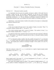
Definition. The complex numbers—denoted by C—are R 2 equipped with the operations
for x,y,u,v ∈ R.
(x,y)+(u,v) := (x+u,y +v),
(x,y)(u,v) := (xu−yv,xv+yu)
Theorem 1.1 (C is a Field). The complex numbers are a field. Specifically, we have:
• (0,0) is the identity element of addition;
• −(x,y) = (−x,−y) for x,y ∈ R;
• (1,0) is the identity element of multiplication;
• (x,y) −1 �
= for x,y ∈ R with (x,y) �= (0,0).
�
x
x2 −y
+y2, x2 +y2 Proof (of the last claim only). Let x,y ∈ R besuch that (x,y) �= (0,0), andnote that
�
x
(x,y)
x2 −y
+y2, x2 +y2 � � 2 x
=
x2 −y2
−
+y2 x2 −xy
+y2, x2 xy
+
+y2 x2 +y2 �
� 2 2 x +y
=
x2 −xy +xy
+y2, x2 +y2 �
= (1,0).
Proposition 1.1. The set {(x,0) : x ∈ R} is a subfield of C, and the map
is an isomorphism onto its image.
θ: R → C, x ↦→ (x,0)
5

6 CHAPTER 1. THE COMPLEX NUMBERS
Proposition 1.1 is often worded as:
R “is” a subfield of C.
Set 1 := (1,0) and i := (0,1). Then, for any z = (x,y) ∈ C, we have
We write
and
z = (x,0)+(0,y) = (1,0)(x,0)+(0,1)(y,0) = x+iy.
Rez := x = “the real part of z”
Imz := y = “the imaginary part of z”.
The complex number i is called the imaginary unit and satisfies
i 2 = (0,1) 2 = (−1,0) = −1.
Unlike R, the set C = {(x,y) : x ∈ R,y ∈ R} is not ordered; there is no notion of
positive and negative (greater than or less than) on the complex plane. For example,
if i were positive or zero, then i 2 = −1 would have to be positive or zero. If i were
negative, then −i would be positive, which would imply that (−i) 2 = i 2 = −1 is
positive. It is thus not possible to divide the complex numbers into of negative, zero,
and positive numbers.
The frequently appearing notation √ −1 for i is misleading and should be avoided,
becausetherule √ xy = √ x √ y (whichonemightanticipate)doesnotholdfornegative
x and y, as the following contradiction illustrates:
1 = √ 1 = � (−1)(−1) = √ −1 √ −1 = i 2 = −1.
Furthermore, bydefinition √ x ≥ 0, butonecannotwritei ≥ 0, sinceCisnotordered.
Definition. For z = x+iy ∈ C, its complex conjugate is defined as ¯z = x−iy.
Proposition 1.2. For z,w ∈ C, the following hold true:
(i) Rez = 1
1
(z + ¯z) and Imz = (z − ¯z);
2 2i
(ii) z +w = ¯z + ¯w;
(iii) zw = ¯z¯w;
(iv) z −1 = ¯z −1 if z �= 0.

Proof. (i): If z = x+iy, then ¯z = x−iy, so that 2x = z+¯z; this yields the claim for
Rez. The assertion for Imz is proven similarly.
(ii) is obvious.
(iii): Let z = x+iy and w = u+iv, so that
and thus
zw = (xu−yv)+i(xv +yu)
zw = (xu−yv)−i(xv +yu).
On the other hand, we have ¯z = x−iy and ¯w = u−iv, which yields
as claimed.
(iv): By (iii), we have
which yields the claim.
¯z¯w = (xu−(−y)(−v))+i(x(−v)+(−y)u)
= (xu−yv)−i(xv +yu)
= zw,
z −1 ¯z = z −1 z = ¯1 = 1,
For any z = x+iy ∈ C, we note that z¯z = x 2 +y 2 ≥ 0. This provides us with a
natural generalization of the absolute value function to C.
Definition. For z ∈ C, set |z|:= √ z¯z.
Proposition 1.3. |·| is the Euclidean norm on R 2 . In particular, the following hold:
(i) |z|≥ 0 with |z|= 0 if and only if z = 0;
(ii) |z +w|≤ |z|+|w| for z,w ∈ C.
Moreover, we have |zw|= |z||w| for z,w ∈ C and z −1 = ¯z
|z| 2 for z ∈ C\{0}.
Proof. Noting that |x+iy|= � x 2 +y 2 , we see that |·| is the Euclidean norm, which
entails (i) and (ii). Letting z,w ∈ C, we see that
|zw| 2 = zwzw = (z¯z)(w¯w) = |z| 2 |w| 2 .
Also, since |z| 2 = z¯z, we have 1 = z ¯z
|z| 2 for z �= 0 and thus z −1 = ¯z
|z| 2.
There is a remarkable similarity between the complex multiplication rule
(x,y)·(u,v) = (xu−yv,xv+yu)
7

8 CHAPTER 1. THE COMPLEX NUMBERS
and the trigonometric angle sum formulae. Notice that
(cosθ,sinθ)·(cosφ,sinφ) = (cosθcosφ−sinθsinφ,cosθsinφ+sinθcosφ)
= (cos(θ+φ),sin(θ+φ)).
Thatis, multiplicationof2complexnumbersontheunitcirclex 2 +y 2 = 1corresponds
to addition of their angles of inclination to the x axis. In particular, the mapping
f(z) = z 2 doubles the angle of z = (x,y) and f(z) = z n multiplies the angle of z
by n. These statements hold even if z lies on a circle of radius r �= 1:
this is known as deMoivre’s Theorem.
(rcosθ,rsinθ) n = r n (cosnθ,sinnθ);

Chapter 2
Complex Differentiation
Definition. Let D ⊂ C, and let z0 be an interior point of D, i.e. there exists ǫ > 0
such that Bǫ(z0) := {z ∈ C : |z − z0|< ǫ} ⊂ D. A function f : D → C is called
complex differentiable at z0 if
exists.
f ′ f(z)−f(z0)
(z0) := lim
z→z0 z −z0
Proposition 2.1. Let D ⊂ C, let z0 ∈ intD, and let f: D → C be complex differentiable
at z0. Then f is continuous at z0.
f(z)−f(z0)
Proof. Since lim
z→z0 z −z0
f(z)−f(z0)
0 = lim(z
−z0) lim
z→z0 z→z0 z −z0
so that f(z0) = lim f(z).
z→z0
exists, we have
= lim(z
−z0)
z→z0
f(z)−f(z0)
z −z0
= lim(f(z)−f(z0)),
z→z0
Proposition 2.2. Let D ⊂ C, and let f,g : D → C be complex differentiable at
z0 ∈ intD. Then the following functions are complex differentiable at z0: f +g, fg,
and, if g(z0) �= 0, f
g
and
. Moreover, we have:
(f +g) ′ (z0) = f ′ (z0)+g ′ (z0),
(fg) ′ (z0) = f ′ (z0)g(z0)+f(z0)g ′ (z0),
� � ′
f
g
(z0) = f′ (z0)g(z0)−f(z0)g ′ (z0)
g(z0) 2
.
9

10 CHAPTER 2. COMPLEX DIFFERENTIATION
Proof. As over R.
Proposition 2.3. Let D,E ⊂ C, let g : D → C and f : E → C be such that
g(D) ⊂ E, and let z0 ∈ intD be such that w0 := g(z0) ∈ intE. Further, suppose
that g is complex differentiable at z0 and f is complex differentiable at w0. Then f◦g
is complex differentiable at z0 with
Proof. As over R.
Examples.
(f ◦g) ′ (z0) = f ′ (g(z0))g ′ (z0).
1. All constant functions are (on all of C) complex differentiable, as is z ↦→ z on
C. Consequently, all complex polynomials are complex differentiable on all of
C, and rational functions are complex differentiable wherever they are defined.
2. Let
f: C → C, z ↦→ ¯z,
and let z0 = x0+iy0 ∈ C. Assume that f is complex differentiable at z0. Then
we have
as well as
f ′ ¯z − ¯z0
(z0) = lim
z→z0
z −z0
(x0 −iy)−(x0 −iy0)
= lim
y→y0 (x0 +iy)−(x0 +iy0)
i(y0 −y)
= lim
y→y0 i(y −y0)
= −1
f ′ ¯z − ¯z0
(z0) = lim
z→z0
z −z0
(x−iy0)−(x0 −iy0)
= lim
x→x0 (x+iy0)−(x0 +iy0)
x−x0
= lim
x→x0 x−x0
= 1,
which is impossible. Hence, f is not complex differentiable at any z0 ∈ C. (On
the other hand, f is continuously partially differentiable—as a function of two
real variables—on all of C.)
Lemma 2.1. The following are equivalent for an R-linear map T : C → C:

(i) there exists c ∈ C such that T(z) = cz for all z ∈ C;
(ii) T is C-linear;
(iii) T(i) = iT(1);
(iv) the real 2×2 matrix representing T with respect to the standard basis of R2 may
be written as
� �
a b
A =
−b a
for some real a,b ∈ R.
Proof. (i) =⇒ (ii) =⇒ (iii) is obvious.
(iii) =⇒ (i): Set c := T(1). For z = x+iy ∈ C, this means that
T(x+iy) = T(x)+T(iy)
= xT(1)+yT(i)
= xT(1)+iyT(1)
= zT(1)
= cz.
(iv) ⇐⇒ (iii): Let a,b,c,d ∈ R be such that
A =
� a b
c d
represents T with respect to the standard basis of R2 . Note that
� �� � � �
a b 1 a
T(1) = = = a+ic,
c d 0 c
and
Since
we see that
T(i) =
� a b
c d
�� 0
1
�
=
�
.
� b
d
iT(1) = −c+ia,
�
= b+id.
T(i) = iT(1) ⇐⇒ c = −b and d = a.
Theorem 2.1 (Cauchy–Riemann Equations). Let D ⊂ C be open, and let z0 ∈ D.
Let f: D → C and denote u := Ref, v := Imf. Then the following are equivalent:
(i) f is complex differentiable at z0;
11

12 CHAPTER 2. COMPLEX DIFFERENTIATION
(ii) f is totally differentiable at z0 (in the sense of multivariable calculus), and the
Cauchy–Riemann differential equations
hold.
Proof. (i) =⇒ (ii): Define
∂u
∂x (z0) = ∂v
∂y (z0) and
T: C → C, z ↦→ f ′ (z0)z,
∂u
∂y (z0) = − ∂v
∂x (z0)
and note that
�
|f(z)−f(z0)−T(z −z0)| �
= �
f(z)−f(z0)
|z −z0| � −f
z −z0
′ �
�
(z0) �
� → 0
as z → z0. Therefore, f is totally differentiable at z0. From multivariable calculus, it
follows that the matrix representation of T with respect to the standard basis of R is
the Jacobian of f, i.e. � �
ux(z0) uy(z0)
Jf(z0) = .
vx(z0) vy(z0)
Since T is C-linear, Lemma 2.1 yields that
ux(z0) = vy(z0) and uy(z0) = −vx(z0).
(ii) =⇒ (i): Since f is totally differentiable at z0, we have a unique R-linear map
T : C → C such that
|f(z)−f(z0)−T(z −z0)|
lim
= 0.
z→z0 |z −z0|
Asweknowfrommultivariablecalculus, T isrepresented byJf(z0)withrespect tothe
standard basis of R2 . Since the Cauchy–Riemann differential equations are supposed
to hold, Jf(z0) is of the form described in Lemma 2.1(iv). By Lemma 2.1, there thus
exists c ∈ C such that T(z) = cz for all z ∈ C. It follows that
� �
�
�
f(z)−f(z0) �
� −c�
z � −z0
= |f(z)−f(z0)−c(z −z0)|
→ 0
|z −z0|
as z → z0. Hence, f is complex differentiable at z0.
Remark. In the situation of Theorem 2.1, we have
f ′ � �� �
ux(z0) uy(z0) 1
(z0)1 =
= ux(z0)+ivx(z0)
vx(z0) vy(z0) 0
as well as
so that
f ′ (z0)i =
� ux(z0) uy(z0)
vx(z0) vy(z0)
�� 0
1
�
= uy(z0)+ivy(z0),
f ′ (z0) = ux(z0)+ivx(z0) = vy(z0)−iuy(z0).

Example. Let
Then f is totally differentiable, with
f: C → C, z ↦→ |z| 2 .
ux = 2x, uy = 2y, vx = vy = 0,
noting that v = 0. The Cauchy–Riemann equations
ux(z0) = vy(z0) and uy(z0) = −vx(z0)
thus hold if and only if z0 = 0. By Theorem 2.1, this means that f is complex
differentiable at z0 if and only if z0 = 0.
Corollary 2.1.1. Let D ⊂ C be open and connected, and let f: D → C be complex
differentiable. Then f is constant on D if and only if f ′ ≡ 0.
Proof. Suppose that f ′ ≡ 0. From the remark after Theorem 2.1, it follows that
ux = vx = uy = vy ≡ 0.
Multivariable calculus then yields that f is constant.
13

Chapter 3
Power Series
Definition. A(complex)power seriesisaninfiniteseriesoftheform �∞ n
n=0an(z−z0) withz,z0,a0,a1,a2,... ∈ C. Thepointz0 iscalledthepoint of expansionfortheseries.
Examples.
1. For m ∈ N, we have
m�
n=0
z n = 1−zm+1
1−z
if z �= 1. For |z|< 1, we obtain (letting m → ∞)
2. For z ∈ C, define
Let z �= 0, and note that
∞�
n=0
z n = 1
1−z .
exp(z) :=
�
�
�
z
�
n+1
��
����
�
�
z
(n+1)! �
n
�
�
�
n! �
∞�
n=0
z n
n! .
= |z|
n+1
→ 0
as n → ∞. As the ratio test holds for series with summands in C as well as for
series over R, we conclude that exp(z) converges absolutely.
Let z,w ∈ C, and note that the Cauchy product formula for series over R also
14

holds over C. We obtain:
�
∞�
z
exp(z)exp(w) =
j=0
j
��
∞�
j!
k=0
∞� n� z
=
n=0 k=0
n−k
(n−k)!
∞� n�
�
1 n
=
n! k
n=0 k=0
n� (z +w)
=
n
n!
n=0
= exp(z +w).
wk �
k!
w k
k!
�
z n−k w k
15
by the Cauchy product formula, letting n = j +k,
We call exp: C → C the exponential function. The above property suggests
using the shorthand e z for exp(z). An interactive three-dimensional graph of
exp(z) is shown in Figure 3.1.
3. The sine and cosine functions on C are defined as
and
sin(z) :=
cos(z) :=
∞�
n=0
(−1) n z 2n+1
(2n+1)!
∞�
(−1)
n=0
n z2n
(2n)!
for z ∈ C. As for exp(z), we see that both sin(z) and cos(z) converge absolutely
for all z ∈ C. Moreover, we have for z ∈ C:
e iz ∞� (iz)
=
n=0
n
n!
∞� (iz)
=
n=0
2n
(2n)! +
∞� (iz)
n=0
2n+1
(2n+1)!
∞�
n z2n
= (−1)
(2n)! +i
∞�
(−1) n z2n+1 (2n+1)!
n=0
= cos(z)+isin(z).
Interactive three-dimensional graphs of the complex cosine and sine functions
are shown in Figures 3.2, and 3.3.
n=0

16 CHAPTER 3. POWER SERIES
Figure 3.1: Surface plot of exp(z) in the complex plane, using an RGB color wheel
to represent the phase. Red indicates real positive values.
Theorem 3.1 (Radius of Convergence). Let � ∞
n=0 an(z − z0) n be a complex power
series. Then there exists a unique R ∈ [0,∞] with the following properties:
• � ∞
n=0 an(z −z0) n converges absolutely at each z ∈ BR(z0);
• for each r ∈ [0,R), the series � ∞
n=0 an(z−z0) n converges uniformly on Br[z0] :=
{z ∈ C : |z −z0|≤ r};
• � ∞
n=0 an(z −z0) n diverges for each z /∈ BR[z0].
Moreover, R can be computed via the Cauchy–Hadamard formula:
R =
1
�
n
limsup |an|
n→∞
.
It is called the radius of convergence for � ∞
n=0 an(z −z0) n .

Figure 3.2: Surface plot of cos(z) in the complex plane, using an RGB color wheel to
represent the phase. Red indicates real positive values.
Proof. The uniqueness of R follows from the first and the last property.
Let R ∈ [0,∞] be defined by the Cauchy–Hadamard formula (we set 1
= ∞ and 0
1 = 0). ∞
Let r ∈ [0,R), and choose r ′ ∈ (r,R). It follows that
�
n
limsup |an| =
n→∞
1 1
<
R r ′,
so that there exists n0 ∈ N such that n� |an| < 1
r ′ whenever n ≥ n0, i.e.
�
1
|an|<
r ′
�n for all n ≥ n0. For n ≥ n0 and z ∈ Br[z0], we then have
|an(z −z0) n �
r
|≤
r ′
�n .
17

18 CHAPTER 3. POWER SERIES
Figure 3.3: Surface plot of sin(z) in the complex plane, using an RGB color wheel to
represent the phase. Red indicates real positive values.
Since r
r ′ < 1, we have �∞ � ∞
n=0
�
r
r ′
�n < ∞. The Weierstraß M-test thus yields that
n=0 an(z −z0) n converges absolutely and uniformly on Br[z0].
Since every z ∈ BR(z0) is contained in Br[z0] for some r ∈ [0,R), it follows that
� ∞
n=0 an(z −z0) n converges absolutely for each such z.
Let z /∈ BR[z0], i.e. |z −z0|> R, so that
1 1
<
|z −z0| R
and thus, for infinitely many n ∈ N,
or, equivalently,
= limsup
n→∞
1
|z −z0| < n� |an|
1 < |an(z −z0) n |.
�
n
|an|

It follows that {an(z−z0) n } ∞ n=1 does not converge to zero. Consequently, � ∞
n=0 an(z−
z0) n diverges.
Examples.
1. � ∞
n=0 zn : R = 1.
2. � ∞
n=0
zn : R = ∞. n!
3. � ∞
n=0 n!zn : R = 0.
4. �∞ z2n+1
n=0 (−1)n (2n+1)! and �∞ z2n
n=0 (−1)n : R = ∞. (2n)!
Theorem 3.2 (Term-by-Term Differentiation). Let � ∞
n=0 an(z − z0) n be a complex
power series with radius of convergence R. Then
f: BR(z0) → C, z ↦→
∞�
an(z −z0) n
n=0
is complex differentiable at each point z ∈ BR(z0) with
f ′ (z) =
∞�
nan(z −z0) n−1 .
n=1
Proof. Without loss of generality, suppose that z0 = 0.
We first show that � ∞
> limsup
n→∞
19
n=1nanz n−1 converges absolutely for each z ∈ BR(0).
�
n
|an|,
Let z ∈ BR(0), and choose r such that |z|< r < R. Since 1
r
there exists n0 ∈ N such that |an|< � �
1 n
for n ≥ n0 and thus
r
|nanz n−1 |< n
� �n−1 |z|
r r
for n ≥ n0. Since |z|
r < 1, we know from the Ratio Test that �∞ n
n=1 r
the Comparison Test then yields that � ∞
n=1 nanz n−1 converges absolutely.
In view of the foregoing, we may define
g: BR(0) → C, z ↦→
∞�
nanz n−1 .
n=1
� �n−1 |z|
< ∞; r
We shall devote the rest of the proof to showing that f is complex differentiable on
BR(0) with f ′ = g.
To this end, fix ǫ > 0, and define, for z ∈ BR(0) and n ∈ N,
Sn(z) :=
n�
akz k
k=0
and Rn(z) :=
∞�
k=n+1
akz k .

20 CHAPTER 3. POWER SERIES
Fix z ∈ BR(0) and let r ∈ (0,R) be such that z ∈ Br(0). Note that
�
f(w)−f(z) Sn(w)−Sn(z)
−g(z) = −S
w −z w−z
′ �
n(z) +(S ′ n(z)−g(z))+ Rn(w)−Rn(z)
w−z
for all w ∈ BR(0)\{z}. We shall see that each of the three summands on the righthand
side of this equation has modulus less than ǫ
, provided that n is sufficiently
3
large and w is sufficiently close to z.
We start with the last summand. First, note that
Rn(w)−Rn(z)
w −z
for all w ∈ BR(0)\{z} and also that
� �
� �
� �
� � =
�
� k� �
�
�
w k −z k
w −z
j=1
=
w k−j z j−1
∞�
k=n+1
�
�
�
�
� ≤
k�
j=1
w
ak
k −zk w −z
|w| k−j |z| j−1 ≤ kr k−1
for all w ∈ Br(0)\{z}. Since r < R, we have �∞ k=1k|ak|r k−1 < ∞. Consequently,
there exists n1 ∈ N such that �∞ k=n+1k|ak|r k−1 < ǫ
3 for all n ≥ n1 and therefore
� �
�
�
Rn(w)−Rn(z) �
�
� w−z � =
�
�
�
�
�
∞�
k=n+1
ak
w k −z k
w −z
�
�
�
�
� ≤
∞�
k=n+1
k|ak|r k−1 < ǫ
3
for all n ≥ n1 and all w ∈ Br(0)\{z}.
For the second summand, just note that lim S
n→∞ ′ n(z) = g(z); consequently, there
exists n2 ∈ N such that |S ′ ǫ
n (z)−g(z)|< for all n ≥ n2.
3
For the first summand, fix n ≥ max{n1,n2}. Since
Sn(w)−Sn(z)
lim
w→z w −z
there exists δ ∈ (0,r) such that
�
�
�
Sn(w)−Sn(z)
� w−z
−S ′ n (z)
= S ′ n (z),
for all w ∈ Bδ(z) ⊂ Br(0)\{z}. Consequently, we obtain for all w ∈ Bδ(z)\{z} that
� �
�
�
f(w)−f(z) �
� −g(z) �
w−z � ≤
�
�
�
Sn(w)−Sn(z)
� −S
w −z
′ n (z)
�
�
�
� +|S′ n (z)−g(z)|+
� �
�
�
Rn(w)−Rn(z) �
�
ǫ
� w−z � <
3 +ǫ
3 +ǫ = ǫ.
3
�
�
�
�
< ǫ
3
Since ǫ > 0 was arbitrary, we see that f ′ (z) exists and equals g(z).

Problem 3.1. Show in Theorem 3.2 that the power series for f ′ and f have the same
radius of convergence.
Examples.
1. exp ′ (z) = exp(z).
2. sin ′ (z) = cos(z).
3. cos ′ (z) = −sin(z).
Corollary 3.2.1 (Higher Derivatives of Power Series). Let � ∞
n=0 an(z − z0) n be a
complex power series with radius of convergence R. Then
f: BR(z0) → C, z ↦→
∞�
an(z −z0) n
n=0
is infinitely often complex differentiable on BR(z0) with
f (k) (z) =
∞�
n(n−1)···(n−k +1)an(z −z0) n−k .
n=k
for z ∈ BR(z0) and k ∈ N. In particular, when z = z0 we see that
holds for each n ∈ N0.
an = 1
n! f(n) (z0)
Corollary 3.2.2 (Integration of Power Series). Let � ∞
n=0 an(z −z0) n be a complex
power series with radius of convergence R. Then
F: BR(z0) → C, z ↦→
is complex differentiable on BR(z0) with
for z ∈ BR(z0).
F ′ (z) =
∞�
n=0
∞�
an(z −z0) n
n=0
an n+1
(z −z0)
n+1
21

Chapter 4
Complex Line Integrals
We call a function f : [a,b] → C integrable if Ref,Imf : [a,b] → R are integrable in
the sense of real variables. (The Riemann integral will do.) In this case, we define
� b � b
f(t)dt :=
a
a
� b
Ref(t)dt+i Imf(t)dt.
a
Definition. A curve (or path) in C is a continuous map γ: [a,b] → C. We call
• γ(a) the initial point of γ,
• γ(b) the endpoint (or terminal point) of γ, and
• {γ} := γ([a,b]) the trajectory of γ.
Collectively, we call γ(a) and γ(b) the endpoints of γ.
Examples.
1. Let z,w ∈ C. Then
γ: [0,1] → C, t ↦→ z0 +t(z −z0)
has the initial point z0 and the endpoint z, and {γ} is the line segment connecting
z0 with z.
2. For k ∈ Z, let
γk: [0,2π] → C, θ ↦→ e ikθ .
Then γk(0) = 1 = γk(2π) holds, and for k �= 0, we have {γk} = {z ∈ C : |z|= 1}.
Definition. A curve γ: [a,b] → C is called piecewise smoothif there exists a partition
a = a0 < a1 < ··· < an = b such that γ|[aj−1,aj] is continuously differentiable for
j = 1,...,n.
22

Definition. The length of a piecewise smooth curve γ: [a,b] → C is defined as
ℓ(γ) :=
n�
� aj
|γ ′ (t)|dt,
j=1
where a = a0 < a1 < ··· < an = b is a partition such that γ|[aj−1,aj] is continuously
differentiable for j = 1,...,n.
Definition. Let γ: [a,b] → C be a piecewise smooth curve, let a = a0 < a1 < ··· <
an = b beapartitionsuch that γ|[aj−1,aj] iscontinuously differentiable forj = 1,...,n,
and let f : {γ} → C be continuous. Then the line integral (or contour integral) of f
along γ is defined as
�
γ
�
f :=
γ
f(ζ)dζ =
aj−1
n�
� aj
j=1
aj−1
f(γ(t))γ ′ (t)dt.
Properties of the Line Integral. 1. Let γ be a piecewise smooth curve, let
λ,µ ∈ C, and let f,g: {γ} → C be continuous. Then we have
� � �
(λf +µg) = λ f +µ g.
γ
2. Let γ be a piecewise smooth curve, let f : {γ} → C be continuous, and let
C ≥ 0 be such that |f(ζ)|≤ C for ζ ∈ {γ}. Then
��
�
� �
�
� f�
� ≤ Cℓ(γ)
holds.
γ
3. Let γ : [c,d] → C be a piecewise smooth curve, let φ : [a,b] → [c,d] be a
continuously differentiable function with φ(a) = c and φ(b) = d, and let f :
{γ} → C be continuous. Then we have
� �
f = f.
γ
4. Let D ⊂ C be open, and let f : D → C be continuous with antiderivative
F : D → C; i.e. F is complex differentiable at each z ∈ D, with F ′ (z) = f(z).
Then �
f = F(γ(b))−F(γ(a))
γ
γ◦φ
holds for every piecewise smooth curve γ: [a,b] → D.
γ
γ
23

24 CHAPTER 4. COMPLEX LINE INTEGRALS
Definition. A curve γ: [a,b] → C is called closed if γ(a) = γ(b).
Proposition 4.1. Let D ⊂ C be open, and let f : D → C be continuous with an
antiderivative. Then �
f = 0 holds for each closed, piecewise smooth curve γ in D.
Example. Let z0 ∈ C, let r > 0, and let
γ
γ: [0,2π] → C, θ ↦→ re iθ +z0,
i.e. γ is a counterclockwise-oriented circle centered at z0 with radius r.
Let n ∈ Z, and consider �
γ (ζ −z0) ndζ. For n �= −1, let
n+1 (z −z0)
F : C → C, z ↦→ ,
n+1
so that F ′ (z) = (z −z0) n for all z ∈ C. It follows that �
On the other hand, we have
Consequently,
�
has no antiderivative.
γ
(ζ −z0) −1 dζ =
� 2π
0
γ (ζ −z0) n dζ = 0.
rieiθ � 2π
dθ = idt = 2πi.
reiθ 0
C\{z0} → C, z ↦→ 1
z −z0
Recall the following definition from multivariable calculus:
Definition. A subset D ⊂ C is called connected if there are no open sets U,V ⊂ C
with
• U ∩D �= ∅ �= V ∩D;
• U ∪V ⊃ D;
• U ∩V ⊂ C\D.
In other words, there are no open sets U and V, each containing points of D, such
that every point of D lies in exactly one of the sets U and V.
Definition. Let D ⊂ C be open. A function f : D → C is called locally constant if,
for each z0 ∈ D, there exists ǫ > 0 such that Bǫ(z0) ⊂ D and f is constant on Bǫ(z0).
The following curve constructions will be useful in understanding the relation
between locally constant functions and connectivity.

1. Given a < b < c and two curves γ1 : [a,b] → C and γ2 : [b,c] → C with
γ1(b) = γ2(b), the concatenation of γ1 and γ2 is the curve
�
γ1(t), t ∈ [a,b],
γ1 ⊕γ2: [a,c] → C, t ↦→
γ2(t), t ∈ [b,c].
If γ1 and γ2 are piecewise smooth, then so is γ1 ⊕γ2, and we have
�
γ1⊕γ2
�
f =
for each continuous f: {γ1}∪{γ2} → C.
γ1
�
f +
2. For any curve γ: [a,b] → C, the reversed curve is defined as
γ − : [a,b] → C, t ↦→ γ(a+b−t).
If γ is piecewise smooth, then so is γ− , and we have
� �
f = − f
for each continuous f: {γ} → C.
γ −
3. We denote the straight line segment {z0 +t(z −z0) : t ∈ [0,1]} by [z0,z].
Proposition 4.2 (Locally Constant vs. Connectivity). Let D ⊂ C be open. Then
the following are equivalent:
(i) D is connected;
(ii) every locally constant function f: D → C is constant;
(iii) for any z,w ∈ D, there exists a piecewise smooth curve γ: [a,b] → D such that
γ(a) = z and γ(b) = w.
Proof. (iii) =⇒ (ii): Let f: D → C be a locally constant function, and let z,w ∈ D.
Let γ: [a,b] → D be a piecewise smooth curve with γ(a) = z and γ(b) = w. Since f
is locally constant, the function
γ
γ2
[a,b] → C, t ↦→ f(γ(t))
is differentiable with zero derivative and therefore constant. It follows that f(z) =
f(γ(a)) = f(γ(b)) = f(w).
(ii) =⇒ (i): Suppose that D is not connected. Then there exist non-empty open
sets U,V ⊂ C with U ∩V = ∅ and U ∪V = D. Define
f: D → C, z ↦→
f
� 0, z ∈ U,
1, z ∈ V.
25

26 CHAPTER 4. COMPLEX LINE INTEGRALS
Then f is locally constant, but not constant.
(i) =⇒ (iii): Let z ∈ D, and set
U := {w ∈ D : ∃ a piecewise smooth curve γ: [a,b] → D with γ(a) = z, γ(b) = w}.
Obviously, U �= ∅ (because z ∈ U).
We claim that U is open. To see this, let w0 ∈ U, so that there exists a piecewise
smooth curve γ: [a,b] → D with γ(a) = z and γ(b) = w0. Choose ǫ > 0 such that
Bǫ(w0) ⊂ D. For w ∈ Bǫ(w0), we know that [w0,w] is a curve in Bǫ(w0) ⊂ D with
initial point w0 and endpoint w. Consequently, γ ⊕ [w0,w] is a piecewise smooth
curve in D with initial point z and endpoint w. It follows that w ∈ U, and since
w ∈ Bǫ(w0) was arbitrary, we have Bǫ(w0) ⊂ U. This proves the openness of U.
Next, we claim that D \ U is also open. To see this, let w0 ∈ D \ U, and let
ǫ > 0 be so small that Bǫ(w0) ⊂ D. Assume towards a contradiction that there exists
w ∈ Bǫ(w0)∩U. Let γ: [a,b] → D be a piecewise smooth curve with γ(a) = z and
γ(b) = w. Then γ⊕[w,w0] is a piecewise smooth curve in D with initial point z and
endpoint w0, so that w0 ∈ U. This contradicts the choice of w0 ∈ D \U. It follows
that Bǫ(w0)∩U = ∅, i.e. Bǫ(w0) ⊂ D \U.
Since U and D \U are both open with U ∪(D \U) = D and U ∩(D \U) = ∅,
the connectedness of D yields that D\U = ∅, i.e. D = U.
Lemma 4.1. Suppose D ⊂ C is an open connected set (a region) and f : D → C is
continuous. Let z0 ∈ D. For each z ∈ D, let γz : [a,b] → D be a piecewise smooth
curve in D such that γz(a) = z0 and γz(b) = z. Consider the function
�
F: D → C, z ↦→ f(ζ)dζ.
For each z, let δ > 0 such that Bδ(z) ⊂ D. If the condition
�
F(w)−F(z) = f(ζ)dζ
γz
[z,w]
holds for each z and all w ∈ Bδ(z), then F is an antiderivative for f.
Proof. Let z ∈ D. Given ǫ > 0, choose δ > 0 small enough such that Bδ(z) ⊂ D and
For all w ∈ Bδ(z), we find
� �
�
�
F(w)−F(z) �
� −f(z) �
w −z � =
|ζ −z|< δ ⇒ |f(ζ)−f(z)|< ǫ.
=
��
1 �
�
|w−z| �
��
1 �
�
|w−z| �
[z,w]
[z,w]
� �
�
f − f(z) �
�
[z,w]
�
�
(f −f(z)) �
�
≤ |w−z|
|w−z| sup{|f(ζ)−f(z)|: ζ ∈ {[z,w]}}
= sup{|f(ζ)−f(z)|: ζ ∈ {[z,w]}} < ǫ.

That is, F ′ (z) = f(z).
Theorem 4.1 (Antiderivative Theorem). Let D ⊂ C be open and connected and let
f: D → C be continuous. Then the following are equivalent:
(i) f has an antiderivative;
(ii) �
f(ζ)dζ = 0 for any closed, piecewise smooth curve γ in D;
γ
(iii) for any piecewise smooth curve γ in D, the value of �
f depends only on the
γ
inital point and the endpoint of γ.
Proof. (i) =⇒ (ii) is Proposition 4.1.
(ii) =⇒ (iii): Let γ,Γ: [a,b] → D be piecewise smooth curves with γ(a) = Γ(a)
and γ(b) = Γ(b). Then γ ⊕Γ− is a closed, piecewise smooth curve, so that
� � � � �
0 = f = f + f = f − f.
γ⊕Γ −
γ
(iii) =⇒ (i): Fix z0 ∈ D. For each z ∈ D, choose a piecewise smooth curve
γz : [a,b] → D with γz(a) = z0 and γz(b) = z and let
�
F: D → C, z ↦→ f(ζ)dζ.
For each z ∈ D, choose δ > 0 such that Bδ(z) ⊂ D and note for w ∈ Bδ(z) that
�
F(w) = f(ζ)dζ
γw �
= f(ζ)dζ by (iii)
γz⊕[z,w]
� �
= f(ζ)dζ + f(ζ)dζ
γz
�
[z,w]
= F(z)+ f(ζ)dζ.
Γ −
[z,w]
Lemma 4.1 then implies that F is an antiderivative for f.
Fromnowon, weshall use theword curveasshorthandforpiecewise smooth curve.
γz
γ
Γ
27

Chapter 5
Cauchy’s Integral Theorem and
Formula
Definition. Let D ⊂ C be open. If f : D → C is complex differentiable at each
z ∈ D, then we call f holomorphic (or analytic) on D.
Let z1, z2, and z3 be three different points in C. They span a triangle ∆. Its
boundary can be parametrized as a curve with counterclockwise orientation.
We denote this curve by ∂∆.
∆
z1 z2
Theorem 5.1 (Goursat’sLemma). LetD ⊂ C be open, letf: D → C be holomorphic,
and let ∆ ⊂ D be a triangle. Then we have
�
f(ζ)dζ = 0.
∂∆
Proof. First, we note that the result holds trivially whenever z1, z2, and z3 are colinear.
Otherwise, we can split ∆ at its medians into four subtriangles ∆ (1) , ∆ (2) , ∆ (3) ,
and ∆ (4) as shown in the following figure:
28
z3

∆ (4)
∆ (1) ∆ (2)
As the line segments in the interior of ∆ also occur as their reversed paths, we
have
� 4�
�
f = f,
so that
��
�
�
�
∂∆
∂∆
Choose j ∈ {1,2,3,4} such that � � �
that �� ���
�
�
f�
� ≤
∂∆
j=1
4�
��
�
�
�
j=1
∂∆ (j)
∂∆ (j)
�
�
f�
� .
∆ (3)
29
∂∆ (j) f � � is largest, and set ∆1 := ∆ (j) . It follows
� ��
� �
f�
� ≤ 4�
�
also, note that ℓ(∂∆1) = 1
2 ℓ(∂∆).
Repeat this argument with ∆1 in place of ∆, and obtain a triangle ∆2 ⊂ ∆1 with
and �� ���
so that �� ���
∂∆1
�
�
f�
� ;
ℓ(∂∆2) = 1
2 ℓ(∂∆1) = 1
4 ℓ(∂∆)
∂∆
∂∆1
� ��
� �
f�
� ≤ 4�
�
Inductively, we obtain triangles
� ��
� �
f�
� ≤ 4�
�
∂∆1
∂∆2
�
�
f�
� ,
� ��
� �
f�
� ≤ 16�
�
∆ ⊃ ∆1 ⊃ ∆2 ⊃ ···
∂∆2
�
�
f�
� .

30 CHAPTER 5. CAUCHY’S INTEGRAL THEOREM AND FORMULA
with
ℓ(∂∆n) = 1
2nℓ(∂∆) and �� ���
� ��
� �
f�
� ≤ 4n�
�
�
�
f�
�
for n ∈ N.
Let z0 ∈ � ∞
n=1 ∆n, and define
∂∆
∂∆n
r: D → C, z ↦→ f(z)−f(z0)−f ′ (z0)(z −z0),
|r(z)| � �
so that lim = 0 and (r −f) =
z→z0 |z −z0| γ γ [−f(z0)−f ′ (z0)(z −z0)]dz = 0 for each
closed curve γ in D (noting that the integrand has an antiderivative). Consequently,
��
�
�
�
� ��
� �
f�
� ≤ 4n�
�
�
�
r�
�
∂∆
∂∆n
for n ∈ N. Let ǫ > 0 and choose δ > 0 such that
� �
�
�
r(z) �
�
�z
−z0
� ≤
ǫ
[ℓ(∂∆)] 2
for all z ∈ D with |z −z0|< δ. Choose n ∈ N such that ∆n ⊂ Bδ(z0). For z ∈ ∆n,
this means that
|z −z0|≤ ℓ(∂∆n) = 1
2nℓ(∂∆). We thus obtain:
���� � � ��
� �
f�
� ≤ 4n�
�
�
�
r�
�
∂∆
∂∆n
≤ 4 n ℓ(∂∆n) sup
ζ∈∂∆n
≤ 2 n ℓ(∂∆) sup
ζ∈∂∆n
≤ ǫ.
As ǫ > 0 was arbitrary, this proves the claim.
|r(ζ)|= 2 n ℓ(∂∆) sup
ǫ
|ζ −z0|
[ℓ(∂∆)] 2
� �� �
≤ 1
2 nℓ(∂∆)
ζ∈∂∆n
|r(ζ)|
Definition. A set D ⊂ C is called star shaped if there exists z0 ∈ D such that
[z0,z] ⊂ D for each z ∈ D. The point z0 is called a center for D.
Theorem 5.2. Let D ⊂ C be open and star shaped with center z0, and let f: D → C
be continuous such that �
f(ζ)dζ = 0
∂∆
for each triangle ∆ ⊂ D with z0 as a vertex. Then f has an antiderivative.

Proof. Let z0 ∈ D be a center for D. Define
�
F : D → C, z ↦→
Let z ∈ D, and let δ > 0 be such that Bδ(z) ⊂ D. Let w ∈ Bδ(z). Since [z0,z] ⊕
[z,w]⊕[w,z0] is the boundary of a triangle ∆ ⊂ D,
�
f = 0,
so that
�
F(w) =
[z0,w]
[z0,z]⊕[z,w]⊕[w,z0]
[z0,z]
� � � �
f = − f = f + f = F(z)+ f.
[w,z0] [z0,z] [z,w] [z,w]
Lemma 4.1 then implies that F is an antiderivative for f.
Corollary 5.2.1. Let D ⊂ C be open and star shaped, and let f : D → C be
holomorphic. Then f has an antiderivative.
Proof. Apply Goursat’s Lemma and Theorem 5.2.
Corollary 5.2.2. Let D ⊂ C be open, and let f : D → C be holomorphic. Then,
for each z0 ∈ D, there exists a neighbourhood U ⊂ D of z0 such that f|U has an
antiderivative.
Corollary 5.2.3 (Cauchy’s Integral Theorem for Star-Shaped Domains). Let D ⊂ C
be open and star shaped, and let f: D → C be holomorphic. Then �
f(ζ)dζ = 0 for
γ
each closed curve γ in D.
Proof. This follows from Corollary 5.2.1 and Theorem 4.1.
Example. The sliced plane is defined as
f.
C− := {z ∈ C : z /∈ (−∞,0]}.
Then C− is star shaped (1 is a center, for instance). As seen in the proof of Theorem
5.2, the function
�
Log: C− → C, z ↦→
1
ζ dζ
is an antiderivative of z ↦→ 1
z on C−; it is called the principal branch of the logarithm.
Let z ∈ C−, and let γz be any curve in C− with initial point 1 and endpoint z.
From Theorem 4.1, we conclude that �
1
dζ = Logz. γz ζ
For any z ∈ C−, there exists a unique θ ∈ (−π,π)—the principal argument Argz
of z—such that z = |z|eiθ . For z ∈ C−, the curve
[1,z]
γ: [0,θ] → C, t ↦→ |z|e it .
31

32 CHAPTER 5. CAUCHY’S INTEGRAL THEOREM AND FORMULA
has the initial point |z| and the endpoint z. It follows that [1,|z|]⊕γ is curve with
initial point 1 and endpoint z as shown:
It follows that
�
Logz :=
[1,|z|]
y
θ
[1,z]
1 [1,|z|] |z|
� � θ
1 1 |z|e
dζ + dζ = log|z|+i
ζ γ ζ 0
it
dt = log|z|+iArgz.
|z|eit Lemma 5.1. Let D ⊂ C be open and star shaped with center z0, and let f : D → C
be continuous such that f|D\{z0} is holomorphic. Then f has an antiderivative on D.
Proof. Let ∆ be a triangle in D having a vertex z0:
z2
z0 z1 w
Let z1 be an interior point of [z0,w], let z2 be an interior point of [z0,z], and let
z3 be an interior point of [w,z]. As shown above, we use these points to split ∆ into
z
z3
γ
x
z

four subtriangles, denoted by ∆(z0,z1,z2), ∆(z1,z3,z2), ∆(z1,w,z3), and ∆(z2,z3,z).
As in the proof of Goursat’s Lemma, we have
� � � � �
f = f + f + f + f.
∂∆
∂∆(z0,z1,z2)
∂∆(z1,z3,z2)
∂∆(z1,w,z3)
∂∆(z2,z3,z)
Since ∆(z1,z3,z2),∆(z1,w,z3),∆(z2,z3,z) ⊂ D\{z0}, and since f is holomorphic on
D \{z0}, Goursat’s Lemma yields
� � �
f = f = f = 0,
∂∆(z1,z3,z2)
so that �
It follows that
��
�
�
�
∂∆
�
�
f�
� =
��
�
�
�
∂∆(z0,z1,z2)
∂∆
∂∆(z1,w,z3)
�
f =
∂∆(z0,z1,z2)
∂∆(z2,z3,z)
f.
�
�
f�
� ≤ ℓ(∂∆(z0,z1,z2)) sup |f(ζ)|.
ζ∈∂∆(z0,z1,z2)
Since|f|iscontinuouson∆, itisboundedabovebysomeM > 0. Byplacingz1 andz2
sufficiently close to z0, we see that ℓ(∂∆(z0,z1,z2)) can be made smaller than every
ǫ/M > 0. We deduce that �
f = 0. The result then follows from Theorem 5.2.
∂∆
Let z0 ∈ C, and let r > 0. Slightly abusing notation, we use ∂Br(z0) to denote
the boundary of Br(z0) oriented counterclockwise.
Lemma 5.2. Let D ⊂ C be open, let z0 ∈ D, and let r > 0 be such that Br[z0] ⊂ D.
Then �
1
dζ = 2πi
ζ −z
for all z ∈ Br(z0).
∂Br(z0)
Proof. Through direct computation, we saw on pg. 24 that
�
1
dζ = 2πi.
ζ −z0
∂Br(z0)
Let z ∈ Br(z0), and choose ǫ > 0 such that Bǫ[z] ⊂ Br(z0), so that
�
1
dζ = 2πi.
ζ −z
We need to show that
� �
1
dζ =
ζ −z
∂Br(z0)
∂Bǫ(z)
∂Bǫ(z)
�
1
dζ = −
ζ −z ∂Bǫ(z) −
1
ζ −z dζ.
33

34 CHAPTER 5. CAUCHY’S INTEGRAL THEOREM AND FORMULA
This is how the situation looks like:
∂B − ǫ z
We connect the boundaries of Br(z0) and Bǫ(z) through line segments:
Consider the following two closed curves γ1 and γ2:
z0
z0
z

γ1
Then it is clear that
� �
1
dζ +
ζ −z
γ1
γ2
z0
z
�
1
dζ =
ζ −z ∂Br(z0)
z0
z
�
1
dζ +
ζ −z ∂Bǫ(z) −
γ2
1
ζ −z dζ.
The sketches also show that there exist star-shaped open set Dj ⊂ C \ {z} with
{γj} ⊂ Dj for j = 1,2. Cauchy’s integral theorem for star-shaped domains thus
yields that
for j = 1,2, which proves the claim.
�
γj
1
dζ = 0
ζ −z
Theorem 5.3 (Cauchy’s Integral Formula for Circles). Let D ⊂ C be open, let
f: D → C be holomorphic, and let z0 ∈ D and r > 0 be such that Br[z0] ⊂ D. Then
we have
for all z ∈ Br(z0).
f(z) = 1
�
f(ζ)
2πi ∂Br(z0) ζ −z dζ
Remark. A consequence of Theorem 5.3 is that the values of f on all of Br[z0] are
pre-determined by those on ∂Br(z0)!
Proof of Theorem 5.3. Since Br[z0] is compact, we may choose R > 0 be such that
Br[z0] ⊂ BR(z0) ⊂ D. Let z ∈ Br(z0), and note that z is a center for the star-shaped
domain BR(z0).
Define
g: D → C, ζ ↦→
� f(ζ)−f(z)
ζ−z , ζ �= z,
f ′ (z), ζ = z.
35

36 CHAPTER 5. CAUCHY’S INTEGRAL THEOREM AND FORMULA
Then g is continuous on D and holomorphic on D \ {z}. By Lemma 5.1, g has an
antiderivative on BR(z0). Since ∂Br(z0) is closed, this means that
�
0 =
∂Br(z0)
using the identity �
yields the claim.
�
g(ζ)dζ =
∂Br(z0)
∂Br(z0)
�
f(ζ) 1
dζ −f(z)
ζ −z ∂Br(z0) ζ −z dζ,
� �� �
=2πi
1 dζ = 2πi established by Lemma 5.2. Division by 2πi
ζ−z
Corollary 5.3.1 (Mean Value Equation). Let D ⊂ C be open, let f : D → C be
holomorphic, and let z0 ∈ D and r > 0 be such that Br[z0] ⊂ D. Then we have
Proof. Parametrize ∂Br(z0) as
The Cauchy Integral Formula then yields
f(z0) = 1
� 2π
f(z0 +re
2π 0
iθ )dθ.
γ: [0,2π] → C, θ ↦→ z0 +re iθ .
f(z0) = 1
�
2πi
= 1
2πi
= 1
2π
γ
� 2π
0
� 2π
0
f(ζ)
dζ
ζ −z0
f(z0 +re iθ )
re iθ ire iθ dθ
f(z0 +re iθ )dθ.
Lemma 5.3. Let D ⊂ RN be open, and let f: [a,b]×D → R be continuous such that
: [a,b]×D → R all exist and are continuous. Define
∂f ∂f
,..., ∂x1 ∂xN
� b
g: D → R, x ↦→ f(t,x)dt.
Then g is continuously partially differentiable with
for x ∈ D and j = 1,...,N.
� b
∂g ∂f
(x) = (t,x)dt
∂xj ∂xj
a
a

Proof. There is no loss of generality supposing that N = 1.
Let x0,x ∈ D be such that every number between them is also in D. By the
Mean Value Theorem of single variable calculus, there exists, for each t ∈ [a,b], a real
number ξt between x0 and x such that
f(t,x)−f(t,x0)
x−x0
= ∂f
∂x (t,ξt).
Let ǫ > 0. By uniform continuity, there exists a δ > 0 such that
�
�
�
∂f ∂f
� (t,x1)−
∂x ∂x (t,x2)
�
�
�
ǫ
� <
b−a
for any t ∈ [a,b] and all x1,x2 between x0 and x with |x1 −x2|< δ.
Suppose that |x0 −x|< δ. Then we have:
� �
�
b
�
g(x)−g(x0) ∂f
� −
x−x0 a ∂x (t,x0)dt
�
�
�
� =
��
� b�
�
f(t,x)−f(t,x0)
� −
a x−x0
∂f
∂x (t,x0)
� �
�
dt�
�
� � b�
≤ �
f(t,x)−f(t,x0)
� −
a x−x0
∂f
∂x (t,x0)
�
�
�
�dt � � b�
= �
∂f ∂f
� (t,ξt)−
a ∂x ∂x (t,x0)
�
�
�
�dt � b
ǫ
≤
b−a dt, because |ξt −x0|< δ,
= ǫ.
This proves that g is differentiable at x0 with g ′ (x0) = � b
a
A similar (but easier) argument shows that g ′ is continuous.
a
∂f
∂x (t,x0)dt.
Lemma 5.4. Let D ⊂ C be open, and let f: [a,b]×D → C be continuous such that
: [a,b]×D → C exists and is continuous. Define
∂f
∂z
Then g is holomorphic with
for z ∈ D.
� b
g: D → R, z ↦→ f(t,z)dt.
g ′ � b
(z) =
a
a
∂f
∂z (t,z)dt
Proof. Apply Lemma 5.3 to Ref and Imf and note that the Cauchy Riemann differential
equations are satisfied.
37

38 CHAPTER 5. CAUCHY’S INTEGRAL THEOREM AND FORMULA
Theorem 5.4 (Higher Derivatives). Let D ⊂ C be open, let z0 ∈ D and r > 0 be
such that Br[z0] ⊂ D, and let f: D → C be continuous such that
f(z) = 1
�
f(ζ)
2πi ζ −z dζ
∂Br(z0)
holds for all z ∈ Br(z0). Then f is infinitely often complex differentiable on Br(z0)
and satisfies
f (n) (z) = n!
�
f(ζ)
dζ
2πi ∂Br(z0) (ζ −z) n+1
(∗)
holds for all z ∈ Br(z0) and n ∈ N0.
Proof. We prove by induction on n ∈ N0: f is n-times complex differentiable and (∗)
holds.
For n = 0, the claim is clear, so suppose that it is true for some n ∈ N0. Define
F : [0,2π]×Br(z0) → C, (θ,z) ↦→ n!
2π
f(z0 +re iθ )re iθ
(z0 +re iθ −z) n+1.
Then F is continuous and, by the induction hypothesis, satisfies
f (n) (z) = n!
� � 2π
f(ζ)
dζ = F(θ,z)dθ
2πi ∂Br(z0) (ζ −z) n+1
0
for all z ∈ Br(z0). Furthermore,
∂F
∂z
0
(θ,z) = (n+1)!
2π
f(z0 +re iθ )re iθ
(z0 +re iθ −z) n+2
is continuous on [0,2π] × Br(z0). From Lemma 5.4, we thus conclude that f (n) is
holomorphic on D with
f (n+1) � 2π
�
∂F (n+1)! f(ζ)
(z) = (θ,z)dθ = dζ.
∂z 2πi ∂Br(z0) (ζ −z) n+2
Corollary 5.4.1 (Generalized Cauchy Integral Formula). Let D ⊂ C be open, and
let f: D → C be holomorphic. Then f is infinitely often complex differentiable on D.
Moreover, for any z0 ∈ D and r > 0 such that Br[z0] ⊂ D, the generalized Cauchy
integral formula
holds for all z ∈ Br(z0) and n ∈ N0.
f (n) (z) = n!
�
f(ζ)
dζ
2πi ∂Br(z0) (ζ −z) n+1

Proof. Apply Theorem 5.3 and 5.4.
Example. We shall use Cauchy’s integral theorem and formula to evaluate the line
integral
�
eζ ζ(ζ −1) dζ
for various curves γ:
(a) γ = ∂Bπ(−3): The function
γ
f: C\{1} → C, z ↦→ ez
z −1
is holomorphic, and we have Bπ[−3] ⊂ C\{1}. Cauchy’s integral formula thus
yields:
�
(b) γ = ∂B1
2
∂Bπ(−3)
eζ �
f(ζ)
dζ = dζ = 2πif(0) = −2πi.
ζ(ζ −1) ∂Bπ(−3) ζ
(i): As the integrand is holomorphic in the star-shaped domain B3(i),
4
Cauchy’s integral theorem yields that
�
∂B1 (i)
2
eζ dζ = 0.
ζ(ζ −1)
(c) γ = ∂B2(0): the method of partial fractions yields
∂B2(0)
1 1 1
= −
z(z −1) z −1 z .
Since 0,1 ∈ B2(0), we obtain with the help of Cauchy’s integral formula:
�
eζ �
dζ =
ζ(ζ −1)
eζ �
dζ −
ζ −1
eζ dζ = 2πi(e−1).
ζ
∂B2(0)
∂B2(0)
Theorem 5.5 (Characterizations of Holomorphic Functions). Let D ⊂ C be open,
and let f: D → C be continuous. Then the following are equivalent:
(i) f is holomorphic;
(ii) the Morera condition holds, i.e. �
(iii) for each z0 ∈ D and r > 0 with Br[z0] ⊂ D, we have
f(z) = 1
�
f(ζ)
2πi ζ −z dζ
for z ∈ Br(z0);
∂∆
f(ζ)dζ = 0 for each triangle ∆ ⊂ D;
∂Br(z0)
39

40 CHAPTER 5. CAUCHY’S INTEGRAL THEOREM AND FORMULA
(iv) for each z0 ∈ D, there exists r > 0 with Br[z0] ⊂ D and
f(z) = 1
�
f(ζ)
2πi ζ −z dζ
for z ∈ Br(z0);
∂Br(z0)
(v) f is infinitely often complex differentiable on D;
(vi) for each z0 ∈ D, there exists a neighbourhood U ⊂ D of z0 such that f has an
antiderivative on U.
Proof. (i) =⇒ (ii) is Goursat’s Lemma.
(i) =⇒ (iii) is the Cauchy Integral Formula for circles, and (iii) =⇒ (iv) is trivial.
(iv) =⇒(v) followsimmediately fromTheorem 5.4, and(v) =⇒ (i) isagaintrivial.
(ii) =⇒ (vi) follows from Theorem 5.2 because every z0 ∈ D has an open, starshaped
neighbourhood contained in D.
(vi) =⇒ (v): Let z0 ∈ D, and let U ⊂ D be a neighbourhood of z0 such that f
has an antiderivative, say F, on U. Then F is holomorphic on U. Applying (i) =⇒
(v) to F, we see that F is infinitely often complex differentiable on U. Consequently,
f = F ′ is infinitely complex differentiable on U. Since z0 ∈ D was arbitrary, we
conclude that f is infinitely often complex differentiable on D.
We conclude this chapter with Liouville’s Theorem and its application to the
Fundamental Theorem of Algebra.
Definition. A holomorphic function defined on all of C is called entire.
Theorem 5.6 (Liouville’s Theorem). Let f : C → C be a bounded entire function.
Then f is constant.
Proof. We will show that f ′ ≡ 0.
Let C ≥ 0 be such that |f(z)|≤ C for all z ∈ C. Let z ∈ C be arbitrary, and let
r > 0. By the generalized Cauchy integral formula, we have
|f ′ (z)|= 1
2π
��
�
�
�
∂Br(z)
f(ζ)
(ζ −z)
2 dζ
�
�
�
�
1
≤
2π ℓ(∂Br(z))
|f(ζ)| 1
sup ≤
ζ∈∂Br(z) |ζ −z| 2 2π 2πrC
C
=
r2 r .
Letting r → ∞, we obtain f ′ (z) = 0. This completes the proof.
Corollary 5.6.1 (Fundamental Theorem of Algebra). Let p be a non-constant polynomial
with complex coefficients. Then p has a zero.
Proof. Assume that p has no zero. Then the function
f: C → C, z ↦→ 1
p(z)

is entire. Since p is a nonconstant polynomial, we have lim |p(z)|= ∞ and thus
|z|→∞
lim
|z|→∞
|f(z)|= 0. Let R > 0 be such that |f(z)|≤ 1 for |z|> R. Since f is continuous it
is bounded on BR[0], and by the choice of R, it is bounded on C\BR[0], too, and thus
bounded on all of C. By Liouville’s Theorem, f is thus constant, and so is therefore
p, which is a contradiction.
Problem 5.1. Let D ⊂ C be open.
(a) Suppose f : D → C has an antiderivative on D and 0 /∈ f(D). Show that there
exists a holomorphic function g: D → C such that f = exp◦g.
Hint: consider f′ (z)
f(z) .
(b) If D is star shaped, and f: D → C is holomorphic such that 0 /∈ f(D), show that
there exists a holomorphic function g: D → C such that f = exp◦g.
Problem 5.2. Let z0 ∈ C, let r > 0, and let f: Br[z0] → C be continuous such that
f|Br(z0) is holomorphic. Show that
f(z) = 1
�
f(ζ)
2πi ∂Br(z0) ζ −z dζ
for all z ∈ Br(z0). Hint: For θ ∈ (0,1), apply the Cauchy integral formula to
z ↦→ f(θ(z −z0)+z0) on ∂Br
θ (z0); then let θ → 1 − .
41

Chapter 6
Convergence of Holomorphic
Functions
Recall the following definition:
Definition. Let D ⊂ C be open. A sequence (fn) ∞ n=1 of C-valued functions on D is
said to converge uniformly on D to f: D → C if, for each ǫ > 0, there exists N ∈ N
such that |fn(z)−f(z)|< ǫ for all n ≥ N and all z ∈ D.
We recall the following theorem from analysis:
Theorem 6.1 (Uniform Convergence Preserves Continuity). Let D ⊂ C be open, and
let (fn) ∞ n=1 be a sequence of continuous, C-valued functions on D converging uniformly
on D to f: D → C. Then f is continuous.
We now “localize” the notion of uniform convergence:
Definition. Let D ⊂ C be open. Then a sequence (fn) ∞ n=1 of C-valued functions on
D is said to converge locally uniformly on D to f : D → C if, for each z0 ∈ D, there
exists a neighbourhood U ⊂ D of z0 such that (fn|U) ∞ n=1 converges to f|U uniformly
on U.
Proposition 6.1 (Local Uniform Convergence). Let D ⊂ C be open, and let (fn) ∞ n=1
be a sequence of continuous, C-valued functions on D converging locally uniformly on
D to f: D → C. Then f is continuous.
Proof. Let z0 ∈ D, and let U ⊂ D be a neighbourhood of z0 such that fn|U→ f|U
uniformly on U By Theorem 6.1, f|U is continuous. Hence, f is continuous at z0.
Proposition 6.2 (Compact Convergence). Let D ⊂ C be open, and let f,f1,f2,...:
D → C be functions. Then the following are equivalent:
(i) (fn) ∞ n=1 converges to f locally uniformly on D;
42

(ii) for each compact K ⊂ D, the sequence (fn|K) ∞ n=1 converges to f|K uniformly on
K.
Proof. (i) =⇒ (ii): Let K ⊂ D be compact. For each z ∈ K, there exists a neighbourhood
Uz ⊂ D of z such that fn|Uz→ f|Uz uniformly on Uz. Since K is compact,
there exist z1,...,zm ∈ K such that
K ⊂ Uz1 ∪···∪Uzm.
Let ǫ > 0. For each j = 1,...,m, there exists nj ∈ N such that |fn(z)−f(z)|< ǫ for
all n ≥ nj and all z ∈ Uzj . Set N := max{n1,...,nm}. Then |fn(z)−f(z)|< ǫ holds
for all n ≥ N and z ∈ K.
(ii)=⇒(i): Letz0 ∈ D, andletr > 0besuchthatBr[z0] ⊂ D. SinceBr[z0]iscompact,
(fn|Br[z0]) ∞ n=1 converges uniformly on Br[z0] to f|Br[z0]. Trivially, (fn|Br(z0)) ∞ n=1
thus converges uniformly on Br(z0) to f|Br(z0).
Instead of locally uniform convergence, we therefore often speak of compact convergence.
Lemma 6.1. Let D ⊂ C be open, let γ be a curve in D, and let f,f1,f2,...: D → C
be continuous functions such that (fn|{γ}) ∞ n=1 converges to f|{γ} uniformly on {γ}.
Then we have �
γ
�
f(ζ)dζ = lim
n→∞
Proof. Let ǫ > 0, and choose N ∈ N such that
|fn(ζ)−f(ζ)|<
γ
fn(ζ)dζ.
ǫ
ℓ(γ)+1
for all n ≥ N and z ∈ {γ}. For n ≥ N, we thus obtain:
��
� �
� �
� fn � − f�
� =
��
�
� �
� (fn � −f) �
�
γ
γ
γ
≤ ℓ(γ)sup{|fn(ζ)−f(ζ)|: ζ ∈ {γ}}
≤ ǫℓ(γ)
ℓ(γ)+1
< ǫ.
Lemma 6.2. Let D ⊂ C be open, let γ be a curve in D, and let f1,f2,...: D → C be
continuous functions converging compactly to f: D → C. Then f is continuous, and
we have � �
f(ζ)dζ = lim
n→∞
fn(ζ)dζ.
γ
γ
43

44 CHAPTER 6. CONVERGENCE OF HOLOMORPHIC FUNCTIONS
Proof. If γ : [a,b] → C is a curve (and thus continuous) then {γ} = γ([a,b]) is
compact. Hence, Lemma 6.1 applies.
Theorem 6.2 (Weierstraß Theorem). Let D ⊂ C be open, let f1,f2,... : D → C
converges to f : D → C compactly. Then f is
be holomorphic such that (fn) ∞ n=1
holomorphic, and (f (k)
n ) ∞ n=1 converges compactly to f (k) for each k ∈ N.
Proof. By Theorem 6.1, f is continuous.
�
To see that f is holomorphic, let ∆ ⊂ D be a triangle. By Goursat’s Lemma,
∂∆fn(ζ)dζ = 0 holds for all n ∈ N. From Lemma 6.2, we conclude that
� �
f(ζ)dζ = lim fn(ζ)dζ = 0,
n→∞
∂∆
i.e. f satisfies the Morera condition and thus is holomorphic.
Let z0 ∈ D, and let 0 < r < R be such that Br[z0] ⊂ BR(z0) ⊂ BR[z0] ⊂ D. For
any z ∈ Br(z0), we have
|f ′ n (z)−f′ (z)| = 1
2π
Let ǫ > 0, and choose N ∈ N such that
∂∆
��
�
�
fn(ζ)−f(ζ)
�
∂BR(z0) (ζ −z) 2
�
�
dζ�
�
≤ 1
2π ℓ(∂BR(z0))
�
�
sup �
fn(ζ)−f(ζ)
� (ζ −z) 2
�
�
�
�
≤
ζ∈∂BR(z0)
R
(R−r) 2
sup |fn(ζ)−f(ζ)|.
ζ∈∂BR(z0)
|fn(ζ)−f(ζ)|< ǫ (R−r)2
R
for all n ≥ N and ζ ∈ ∂BR(z0). Then it follows from the above estimates that
|f ′ n (z)−f′ (z)|≤ ǫforall n ≥ N andz ∈ Br(z0). Consequently, (f ′ n |Br(z0)) ∞ n=1 converges
to f ′ |Br(z0) uniformly on Br(z0). As z0 ∈ D is arbitrary, this means that (f ′ n) ∞ n=1
converges to f locally uniformly, i.e. compactly, on D.
For higher derivatives, the claim now follows by induction.
Lemma 6.3. Let z0 ∈ C, let r > 0, and let z ∈ Br(z0). Then
1
ζ −z =
∞�
n=0
converges absolutely and uniformly on ∂Br(z0).
1 n
(ζ −z0) n+1(z −z0)

Proof. Let ζ ∈ ∂Br(z0), and note that
1
ζ −z =
1
(ζ −z0)−(z −z0)
= 1
ζ −z0
1
1− z−z0
ζ−z0
�
�
Since |z −z0|< r and |ζ −z0|= r, we have � z−z0
�
�
� < 1, so that
ζ−z0
1
ζ −z =
∞�
� �n 1 z −z0
=
(ζ −z0) ζ −z0 n=0
�
� (z−z0) n
Since � (ζ−z0) n+1
�
�
� =
lute and uniform convergence on ∂Br(z0).
∞�
n=0
1
(ζ −z0) n+1(z −z0) n .
|z−z0| n
rn+1 and �∞ |z−z0|
n=0
n
rn+1 < ∞, the Weierstraß M-test yields abso-
Theorem 6.3 (Power Series for Holomorphic Functions). Let D ⊂ C be open. Then
the following are equivalent for f: D → C:
(i) f is holomorphic;
(ii) for each z0 ∈ D, there exists r > 0 with Br(z0) ⊂ D and a0,a1,a2,... ∈ C such
that f(z) = � ∞
n=0 an(z −z0) n for all z ∈ Br(z0);
(iii) for each z0 ∈ D and r > 0 with Br(z0) ⊂ D, we have
for all z ∈ Br(z0).
f(z) =
∞�
n=0
f (n) (z0)
(z −z0)
n!
n
Proof. (iii) =⇒ (ii) is trivial; (ii) =⇒ (i) follows from Theorem 3.2.
(i) =⇒ (iii): Let z0 ∈ D, and let r > 0 be such that Br(z0) ⊂ D. Let z ∈ Br(z0)
and choose ρ ∈ (0,r) such that z ∈ Bρ(z0). Then we have:
f(z) = 1
�
f(ζ)
2πi ∂Bρ(z0) ζ −z dζ
= 1
� ∞� f(ζ)
2πi ∂Bρ(z0) (ζ −z0)
n=0
n+1(z −z0) n dζ, by Lemma 6.3,
∞�
� � �
1 f(ζ)
=
dζ (z −z0)
2πi
n=0 ∂Bρ(z0) (ζ −z0) n+1 n , by Lemma 6.1,
∞� f
=
(n) (z0)
(z −z0)
n!
n .
n=0
.
45

Chapter 7
Elementary Properties of
Holomorphic Functions
Theorem 7.1 (Identity Theorem). Let D ⊂ C be open and connected, and let f,g:
D → C be holomorphic. Then the following are equivalent:
(i) f = g;
(ii) the set {z ∈ D : f(z) = g(z)} has a cluster point in D;
(iii) there exists z0 ∈ D such that f (n) (z0) = g (n) (z0) for all n ∈ N0.
Proof. Without loss of generality, it suffices to prove the case where g = 0.
(i) =⇒ (iii) is trivial.
(iii) =⇒ (ii): Let z0 ∈ D be as in (iii), and let r > 0 be such that Br(z0) ⊂ D.
Then we have by Theorem 6.3 that
for all z ∈ Br(z0), so that
f(z) =
∞�
n=0
f (n) (z0)
(z −z0)
n!
n = 0
Br(z0) ⊂ Z(f) := {z ∈ D : f(z) = 0}.
Every point in Br(z0) is therefore a cluster point of Z(f).
(ii) =⇒ (i): Let
V := {z ∈ D : z is a cluster point of Z(f)},
so that V �= ∅ by (ii).
We claim that V is open. Let z0 ∈ V, and let r > 0 be such that Br(z0) ⊂ D.
Then
∞�
f(z) = an(z −z0) n
n=0
46

holds for some a0,a1,a2,... ∈ C and all z ∈ Br(z0). As z0 is a cluster point of Z(f),
there exists a sequence (zk) ∞ k=1 in Z(f)\{z0} such that z0 = lim zk. Inductively, we
k→∞
find that an = 0 for all n ∈ N0: given that an = 0 for n = 0,1,2,m−1 we see that
f(zk)
0 = lim
k→∞ (zk −z0) m
∞�
= lim an(zk −z0) n−m = am,
k→∞
n=m
on noting, in view of Theorems 3.1 and 6.3, that the uniform convergence of the
power series on, say, Br/2[z0] justifies the interchange of limits. Hence f(z) = 0 for
all z ∈ Br(z0). That is, Br(z0) ⊂ Z(f) so that Br(z0) ⊂ V.
We now claim that D \V is also open. Let z0 ∈ D \V, and ǫ > 0 be such that
Bǫ(z0) ⊂ D and (Bǫ(z0)\{z0})∩Z(f) = ∅. For any z ∈ Bǫ(z0)\{z0} and δ > 0 such
that Bδ(z) ⊂ Bǫ(z0)\{z0}, we thus have (Bδ(z) \{z}) ∩Z(f) = ∅. It follows that
z /∈ V. Consequently, Bǫ(z0) ⊂ D\V.
In summary, V and D\V are both open and clearly satisfy D = V ∪(D\V) and
V ∩(D \V) = ∅. The connectedness of D yields D = V and thus Z(f) = D.
Examples.
1. There is no non-zero entire function f: C → C such that f � �
1 = 0 for n ∈ N.
n
For any entire function f with this property, 0 is a cluster point of Z(f). By
the Identity Theorem, this means f ≡ 0.
2. Since R has cluster points in C, the holomorphic extensions of exp, cos, and sin
from R to C are unique. For analogous reasons, Log is the only holomorphic
extension of log to C−.
3. There is no entire function f such that
� �
1
f =
n
1
n
and
�
f − 1
�
=
n
1
n2 for n ∈ N. In the view of the identity theorem, the first condition necessitates
that f(z) = z whereas the second one implies that f(z) = (−z) 2 for all z ∈ C.
Lemma 7.1. Let D ⊂ C be open, let f: D → C be holomorphic, and let z0 ∈ D and
r > 0 be such that Br[z0] ⊂ D. Suppose that
Then f has a zero in Br(z0).
|f(z0)|< inf |f(z)|.
z∈∂Br(z0)
47

48CHAPTER7. ELEMENTARYPROPERTIESOFHOLOMORPHICFUNCTIONS
Proof. Assume otherwise, i.e. f has no zero in Br(z0). The hypothesis implies that f
hasno zero on∂Br(z0), so that f has nozero inBr[z0]. Assume however, that foreach
R > 0 such that Br[z0] ⊂ BR(z0) ⊂ D, there is a zero of f in BR(z0). Then we have
a sequence (Rn) ∞ n=1
in (r,∞) with r = lim
n→∞ Rn such that Br[z0] ⊂ BRn(z0) ⊂ D and
Z(f)∩BRn(z0) �= ∅ for each n ∈ N. For each n ∈ N, pick zn ∈ Z(f)∩BRn(z0). Then
(zn) ∞ n=1 is bounded, and thus has a convergent subsequence (znk )∞k=1 with limit z′ .
Clearly, z ′ ∈ Z(f), and since lim Rnk
k→∞ = r, we have z′ ∈ Br[z0], which is impossible.
Consequently, f has no zero on some BR(z0) with Br[z0] ⊂ BR(z0) ⊂ D.
From the Cauchy Integral Formula, we obtain
1
|f(z0)| =
� � �
�
�
1 1 1 �
�
dζ�
2πi ∂Br(z0) f(ζ) ζ � −z0
≤ 1 1
2πr sup
2π ζ∈∂Br(z0) |f(ζ)|r =
1
infζ∈∂Br(z0)|f(ζ)|
and thus
which is a contradiction.
|f(z0)|≥ inf
ζ∈∂Br(z0) |f(ζ)|,
Theorem 7.2 (Open Mapping Theorem). Let D ⊂ C be open and connected, and let
f: D → C be holomorphic and not constant. Then f(D) ⊂ C is open and connected.
Proof. By the continuity of f, it is clear that f(D) is connected.
Let w0 ∈ f(D), and let z0 ∈ D be such that w0 = f(z0). Choose r > 0 such
that Br[z0] ⊂ D and such that {z ∈ Br[z0] : f(z) = w0} = {z0}. (This can be
accomplished with the help of the Identity Theorem.) Let ǫ = 1 inf |f(z)−w0|> 0.
2
∂Br(z0)
We claim that Bǫ(w0) ⊂ f(D). Let w ∈ Bǫ(w0). For z ∈ ∂Br(z0), we have
It follows that
By Lemma 7.1, this means that
|f(z)−w|≥ |f(z)−w0|−|w−w0|> 2ǫ−ǫ = ǫ.
|f(z0)−w|= |w−w0|< ǫ ≤ inf
z∈∂Br(z0) |f(z)−w|.
D → C, z ↦→ f(z)−w
has a zero in Br(z0). It follows that w ∈ f(D).
Theorem 7.3 (Maximum Modulus Principle). Let D ⊂ C be open and connected,
and let f: D → C be holomorphic such that the function
|f|: D → C, z ↦→ |f(z)|
attains a local maximum on D. Then f is constant.

Proof. Let z0 ∈ D be such that |f| attains a local maximum at z0, i.e. there exists
ǫ > 0 such that Bǫ(z0) ⊂ D and |f(z0)|≥ |f(z)| for all z ∈ Bǫ(z0). Then f(z0) is
not an interior point of f(Bǫ(z0)), so that f|Bǫ(z0) is constant by the Open Mapping
Theorem. The Identity Theorem then yields that f is constant.
Corollary 7.3.1. Let D ⊂ C be open and connected, and let f : D → C be holomorphic
such that |f| attains a local minimum on D. Then f is constant or f has a
zero.
Proof. Suppose that f hasno zero. Applying the Maximum Modulus Principle to 1/f
yields that f is constant.
Corollary 7.3.2 (Maximum Modulus Principle for Bounded Domains). Let D ⊂ C
be open, connected, and bounded, and let f: D → C be continuous such that f|D is
holomorphic. Then |f| attains its maximum over D on ∂D.
Proof. The claim is trivial if f is constant, so suppose that f is not constant.
Since f is continuous and D is compact, there exists a point z0 ∈ D with |f(z0)|=
max � |f(z)|: z ∈ D � . If z0 ∈ D, then |f| would attain a local maximum at z0, which
is impossible by the Maximum Modulus Principle. Therefore z0 ∈ ∂D must hold.
From now on, we shall use D to denote the open unit disc B1(0).
Theorem 7.4 (Schwarz’s Lemma). Let f: D → D be holomorphic such that f(0) = 0.
Then one has
|f(z)|≤ |z| for z ∈ D and |f ′ (0)|≤ 1.
Moreover, if there exists z0 ∈ D \ {0} such that |f(z0)|= |z0| or if |f ′ (0)|= 1, then
there exists c ∈ C with |c|= 1 such that f(z) = cz for z ∈ D.
Proof. Let f(z) = � ∞
n=0 anz n be the power series expansion of f. Since f(0) = 0, we
have a0 = 0. Define
g: D → C, z ↦→
∞�
anz n−1 .
Then g is holomorphic with g(0) = a1 = f ′ (0) and f(z) = zg(z) for z ∈ D. Let
r ∈ (0,1). Then we have
|g(z)|= |f(z)| 1
≤
r r
for z ∈ ∂Br(0) andthus for all z ∈ Br[0] by theMaximum Modulus Principle. Letting
r → 1, we deduce that |g(z)|≤ 1 for all z ∈ D and thus |f(z)|≤ |z| for all z ∈ D as
well as |f ′ (0)|= |g(0)|≤ 1.
Suppose that there exists z0 ∈ D\{0} such that |f(z0)|= |z0| or |f ′ (0)|= |g(0)|= 1.
Then |g| has a maximum at z0 or 0, respectively, so that g is constant. Hence, there
exists c ∈ C with |c|= 1 such that f(z) = zg(z) = cz for z ∈ D.
n=1
49

50CHAPTER7. ELEMENTARYPROPERTIESOFHOLOMORPHICFUNCTIONS
Definition. Let D1,D2 ⊂ C be open. Then f: D1 → D2 is called biholomorphic (or
conformal) if
(a) f is bijective and
(b) both f and f −1 are holomorphic.
Corollary 7.4.1. Let f : D → D be biholomorphic such that f(0) = 0. Then there
exists c ∈ C with |c|= 1 such that f(z) = cz for z ∈ D.
Proof. Let z ∈ D. Then |f(z)|≤ |z| holds by Schwarz’s Lemma, as does
|z|= |f −1 (f(z))|≤ |f(z)|.
The result then follows from Schwarz’s Lemma.
Lemma 7.2. Let w ∈ D, and define
Then:
(i) φw maps D bijectively onto D;
(ii) φw(w) = 0;
(iii) φw(0) = w;
(iv) φ −1
w = φw.
φw: D → C, z ↦→
w −z
1− ¯wz .
Proof. Obviously, φw is holomorphic and extends continuously to D.
Then for |z|= 1 we may express
� �
�
|φw(z)|= �
w −z �
�
1
�1−
¯wz � |¯z| =
� �
�
�
w−z �
�
�¯z
− ¯w � = 1.
By the Maximum Modulus Principle, φw(D) ⊂ D holds. Since φw is not constant,
φw(D) is open and thus contained in the interior of D, i.e. in D.
It is obvious that φw(w) = 0 and φw(0) = w.
Moreover, we have for z ∈ D:
(φw ◦φw)(z) =
Hence, φw is bijective with φ −1
w = φw.
= w(1− ¯wz)−(w −z)
w− w−z
1−¯wz
1− ¯w w−z
1−¯wz
(1− ¯wz)− ¯w(w −z)
= −|w|2 z +z
1−|w| 2
= z.

Theorem 7.5 (Biholomorphisms of D). Let f: D → D be biholomorphic. Then there
exist w ∈ D and c ∈ ∂D with f(z) = cφw(z) for z ∈ D.
Proof. Set w := f −1 (0). Then f ◦φw: D → D is biholomorphic with (f ◦φw)(0) = 0.
By Corollary 7.4.1, there exists c ∈ C with |c|= 1 such that f(φw(z)) = cz for z ∈ D,
so that
f(z) = f(φw(φw(z))) = cφw(z)
for z ∈ D.
51

Chapter 8
The Singularities of a Holomorphic
Function
Definition. Let D ⊂ C be open, and let f : D → C be holomorphic. We call
z0 ∈ C\D anisolated singularity of f if there exists ǫ > 0 such that Bǫ(z0)\{z0} ⊂ D.
We say that the isolated singularity z0 is removable if there exists a holomorphic
function g: D ∪{z0} → C such that g|D= f.
Theorem 8.1 (Riemann’s Removability Condition). Let D ⊂ C be open, let f :
D → C be holomorphic, and let z0 ∈ C\D be an isolated singularity of f. Then the
following are equivalent:
(i) z0 is removable;
(ii) there is a continuous function g: D ∪{z0} → C such that g|D= f;
(iii) there exists ǫ > 0 with Bǫ(z0)\{z0} ⊂ D such that f is bounded on Bǫ(z0)\{z0}.
Proof. (i) =⇒ (ii) follows from the continuity of a differentiable function.
(ii) =⇒ (iii) follows from the boundedness of g on a compact set Bǫ[z0] ⊂ D.
(iii) =⇒ (i): Let C ≥ 0 be such that |f(z)|≤ C for z ∈ Bǫ(z0)\{z0}. Define
h: D ∪{z0} → C, z ↦→
� (z −z0) 2 f(z), z �= z0,
0, z = z0.
Then we have for z ∈ Bǫ(z0)\{z0} that
� �
�
�
h(z)−h(z0) �
�
� z −z0
� = |(z −z0)f(z)|≤ C|z −z0|.
Hence, h is holomorphic with h ′ (z0) = h(z0) = 0. Let h(z) = �∞ n=0an(z − z0) n
be the power series representation of h on Bǫ(z0). Then h ′ (z0) = h(z0) = 0 means
that a0 = a1 = 0, so that h(z) = �∞ n=2an(z − z0) n �
for z ∈ Bǫ(z0) and thus f(z) =
∞
n=0an+2(z −z0) n for z ∈ Bǫ(z0)\{z0}.
52

Define
⎧
⎪⎨
g: D ∪{z0} → C, z ↦→
⎪⎩
∞�
an+2(z −z0) n , z ∈ Bǫ(z0),
n=0
Then g is a holomorphic function extending f.
f(z), z ∈ D \Bǫ(z0).
Definition. Let D ⊂ C be open, let f: D → C be holomorphic, and let z0 ∈ C\D
be an isolated singularity of f. Then z0 is called a pole of f if lim|f(z)|=
∞.
z→z0
Example. For n ∈ N, the function
has a pole at 0.
C\{0} → C, z ↦→ 1
z n
Theorem 8.2 (Poles). Let D ⊂ C be open, let f : D → C be holomorphic, and let
z0 ∈ C\D be an isolated singularity of f. Then z0 is a pole of f ⇐⇒ there exist a
unique k ∈ N and a holomorphic function g: D ∪{z0} → C such that g(z0) �= 0 and
for z ∈ D.
f(z) = g(z)
(z −z0) k
Proof.
”⇐” This follows directly from the definition of a pole.
”⇒” Let us prove the uniqueness first. Suppose that there exist natural numbers
k1 ≤ k2 and holomorphic functions g1,g2: D ∪{z0} → C such that gj(z0) �= 0 and
f(z) = gj(z)
(z −z0) kj
for z ∈ D and j = 1,2. If k2 > k1, we then find for all z ∈ D that
g2(z0) = lim
z→z0
g2(z) = lim(z
−z0)
z→z0
k2−k1g1(z) = 0·g1(z0) = 0,
which is a contradiction. Hence k1 = k2 and thus g1 = g2 on D and, by continuity,
on D ∪{z0}.
To establish the existence of k and g, choose r > 0 such that Br(z0)\{z0} ⊂ D
and |f(z)|≥ 1 for all z ∈ Br(z0)\{z0}. Then
Br(z0)\{z0} → C, z ↦→ 1
f(z)
53

54 CHAPTER 8. THE SINGULARITIES OF A HOLOMORPHIC FUNCTION
is holomorphic and bounded and thus, by Riemann’s Removability Criterion, has a
holomorphic extension h: Br(z0) → C with h(z0) = lim 1/f(z) = 0. Note that z0 is
z→z0
the only zero of h. Let
∞�
h(z) = an(z −z0) n
n=0
for z ∈ Br(z0) bethe power series representation of h. Set k := min{n ∈ N0 : an �= 0}.
Since a0 = h(z0) = 0, we have k ≥ 1. Define
˜h: Br(z0) → C, z ↦→
∞�
an(z −z0) n−k .
Then ˜ h is holomorphic, has no zeros, and satisfies h(z) = (z−z0) k˜ h(z) for z ∈ Br(z0).
For z ∈ Br(z0)\{z0}, we thus have
f(z) =
n=k
1
(z −z0) k˜ h(z) ,
so that we can construct the holomorphic function
�
(z −z0)
g: D∪{z0} C, z ↦→
kf(z), z �= z0,
1
˜h(z0)
, z = z0.
Definition. Let D ⊂ C be open, let f: D → C be holomorphic, and let z0 ∈ C\D
be a pole of f. Then the positive integer k in Theorem 8.2 is called the order of z0
and denoted by ord(f,z0). If ord(f,z0) = 1, we call z0 a simple pole of f.
Example. For m ∈ N, consider
fm: C\{0} → C, z ↦→ sinz
.
zm We claim that f1 has a removable singularity at 0 whereas fm has a pole of order
m−1 at 0 for m ≥ 2.
Recall that
sinz =
for z ∈ C. For z �= 0, we thus have
∞�
n=0
f1(z) = sinz
z =
(−1) n z 2n+1
(2n+1)!
∞�
n=0
(−1) n z 2n
(2n+1)! .

Define
g: C → C, z ↦→
∞�
n=0
(−1) n z 2n
(2n+1)! .
Then g is holomorphic and extends f1. Hence, f1 has a removable singularity at 0.
For m ≥ 2 and z �= 0, note that fm(z) = g(z)
zm−1. Since g(0) �= 0, we see that fm has
a pole of order m−1 at 0.
Example. Consider
f: C\{0} → C, z ↦→ e 1
z.
� �
1
Then 0 is not removable because lim f
n→∞ n
for f either: for n ∈ N, we have
�
�
�
�f � ��
i ���
= |e
n
−in |= 1.
55
= lim
n→∞ e n = ∞. But 0 is not a pole
Definition. Let D ⊂ C be open, let f: D → C be holomorphic, and let z0 ∈ C\D
be an isolated singularity of f. Then z0 is called essential if it is neither removable
nor a pole.
Theorem 8.3 (Casorati–Weierstraß Theorem). Let D ⊂ C be open, let f: D → C be
holomorphic, and let z0 ∈ C\D be an isolated singularity of f. Then z0 is essential
⇐⇒ f(Bǫ(z0)∩D) = C for each ǫ > 0.
Proof. “⇐” For each n ∈ N choose zn ∈ B 1
n
follows that lim
n→∞ |f(zn)|= ∞. Hence, z0 cannot be removable.
For each n ∈ N, choose z ′ n
∈ B 1
n
(z0) ∩ D such that |f(zn) − n|< 1.
It n
(z0)∩D such that |f(z ′ n
1 )|< . This means that
lim
n→∞ f(z′ n ) = 0, so that z0 is not a pole either.
“⇒” Assume for some ǫ0 > 0 that f(Bǫ0(z0)∩D) �= C. Without loss of generality,
suppose that Bǫ0(z0) \ {z0} ⊂ D. Let w0 ∈ C and δ > 0 be such that Bδ(w0) ⊂
C\f(Bǫ0(z0)\{z0}). Consider
Then g is holomorphic with
g: Bǫ0(z0)\{z0} → C, z ↦→
|g(z)|=
1
|f(z)−w0|
1
.
f(z)−w0
for z ∈ Bǫ0(z0)\{z0}. Hence, z0 is a removable singularity of g. Let ˜g: Bǫ0(z0) → C
be a holomorphic extension of g.
Case 1: ˜g(z0) �= 0. Since f(z) = 1
˜g(z) + w0 for z ∈ Bǫ0(z0) \ {z0}, this means
that z0 is a removable singularity of f, contradicting the fact that z0 is an essential
singularity.
≤ 1
δ
n

56 CHAPTER 8. THE SINGULARITIES OF A HOLOMORPHIC FUNCTION
Case 2: ˜g(z0) = 0. For z ∈ Bǫ0(z0), we have
�
�
|f(z)|= �
1
�˜g(z)
+w0
�
�
�
1
� ≥
|˜g(z)| −|w0| → ∞.
z→z0
Hence, z0 is a pole of f, again contradicting the fact that z0 is an essential singularity.
Problem 8.1.
Let D ⊂ C be open, let f : D → C be holomorphic, and let z0 ∈ D. Show that the
following are equivalent for n ∈ N:
(i) f (k) (z0) = 0 for k = 0,...,n−1 and f (n) (z0) �= 0;
(ii) there exists a holomorphic function g: D → C with g(z0) �= 0 such that f(z) =
(z −z0) n g(z) for z ∈ D.
If either condition holds, we say that z0 is a zero of f of order n.
Problem 8.2.
Let D ⊂ C be open, let f,g: D → C be holomorphic, and let z0 ∈ D be a zero of
order n for f and of order m ≥ 1 for g. Show the singularity z0 of f
g is
(i) removable if m ≤ n and
(ii) a pole of order m−n otherwise.
Problem 8.3.
Let D ⊂ C be open, let f: D → C be holomorphic, and let z0 ∈ C\D be an isolated
singularity of f.
(a) Show that, if z0 is a pole of order k of f, then it is a pole of order k+1 of f ′ .
(b) Show that exp◦f has either a removable or an essential singularity at z0.

Chapter 9
Holomorphic Functions on Annuli
Definition. Let z0 ∈ C, and let r,R ∈ [0,∞] be such that r < R. Then the annulus
centered at z0 with inner radius r and outer radius R is defined as
Ar,R(z0) := {z ∈ C : r < |z −z0|< R}.
Theorem 9.1 (Cauchy’s Integral Theorem for Annuli). Let z0 ∈ C, let r,ρ,P,R ∈
[0,∞] be such that r < ρ < P < R, and let f : Ar,R(z0) → C be holomorphic. Then
we have � �
f(ζ)dζ = f(ζ)dζ.
∂BP(z0) ∂Bρ(z0)
Proof. The claim is equivalent to
� �
f(ζ)dζ +
Consider
∂BP(z0)
z0
r
∂Bρ(z0) −
57
f(ζ)dζ = 0.
ρ
P
R

58 CHAPTER 9. HOLOMORPHIC FUNCTIONS ON ANNULI
Split∂BP(z0)and∂Bρ(z0) − intofinitelymanyarcsegmentsα1,...,αn andβ1,...,βn,
respectively, andconnectthemwithlinesegmentsγ1,...,γn asshownbelowforn = 3:
We thus obtain
�
∂BP(z0)
α3
�
f(ζ)dζ +
γ − 3
γ3
β3
∂Bρ(z0) −
γ1
γ − 1
β2
α2
f(ζ)dζ =
=
n�
�
j=1
n�
�
j=1
β1
αj
γ − 2
α1
γ2
f(ζ)dζ +
n�
�
j=1
βj
αj⊕γ −
j ⊕βj⊕γ (j+1)mod n
f(ζ)dζ
f(ζ)dζ
Bymakingthearcsegmentsα1,...,αn andβ1,...,βn sufficiently small, wecanensure
that each of the closed curves α1 ⊕γ − 1 ⊕β1 ⊕γ2,...,αn−1 ⊕γ − n−1 ⊕βn−1 ⊕γn,αn ⊕
γ − n ⊕βn ⊕γ1 lies inside a star-shaped open subset of Ar,R(z0):

It follows that
� �
f(ζ)dζ +
∂BP(z0)
as claimed.
∂Bρ(z0) −
f(ζ)dζ
=
n�
�
j=1
αj⊕γ −
j ⊕βj⊕γ (j+1)mod n
f(ζ)dζ = 0
Theorem 9.2 (Laurent Decomposition). Let z0 ∈ C, let r,R ∈ [0,∞] be such that
r < R, and let f : Ar,R(z0) → C be holomorphic. Then there exists a holomorphic
function
g: BR(z0) → C and h: C\Br[z0] → C
with f = g +h on Ar,R(z0). Moreover, h can be chosen such that lim h(z) = 0, in
|z|→∞
which case g and h are uniquely determined.
Proof. We prove the uniqueness assertion first.
Let g1,g2 : BR(z0) → C and h1,h2 : C \ Br[z0] → C be holomorphic such that
lim hj(z) = 0 for j = 1,2 and
|z|→∞
f = g1 +h1 = g2 +h2.
It follows that g1 −g2 = h2 −h1 on Ar,R(z0). Define
F : C → C, z ↦→
� g1(z)−g2(z), z ∈ BR(z0),
h2(z)−h1(z), z ∈ C\Br[z0].
59

60 CHAPTER 9. HOLOMORPHIC FUNCTIONS ON ANNULI
Then F is entire with lim |F(z)|= lim |h2(z) − h1(z)|= 0. Hence, F is bounded
|z|→∞ |z|→∞
andentire and thus constant by Liouville’s theorem. Since lim
|z|→∞
|F(z)|= 0, this means
that F ≡ 0, so that g1 = g2 and h1 = h2.
To show that g and h exists, for z ∈ Ar,R(z0) choose ρ and P such that
Define
r < ρ < |z −z0|< P < R.
G: Ar,R(z0) → C, ζ ↦→
� f(ζ)−f(z)
ζ−z , ζ �= z,
f ′ (z), ζ = z.
ThenGiscertainlyholomorphiconAr,R(z0)\{z}. BecauseitiscontinuousonAr,R(z0),
Riemann’sRemovabilityCriterionimpliesthatGisinfactholomorphiconallofAr,R(z0).
It follows from Cauchy’s Integral Theorem for Annuli that
� �
G(ζ)dζ = G(ζ)dζ,
i.e.
�
∂Bρ(z0)
�
f(ζ)
dζ −f(z)
ζ −z
∂Bρ(z0)
∂Bρ(z0)
1
ζ −z dζ
� �� �
=0
�
=
∂BP(z0)
∂BP(z0)
Let us define the holomorphic functions (cf. Lemma 5.4)
h(z) := −1
�
f(ζ)
2πi ζ −z dζ
on C\Bρ[z0] and
∂Bρ(z0)
g(z) := 1
�
f(ζ)
2πi ∂BP(z0) ζ −z dζ
�
f(ζ) 1
dζ −f(z)
ζ −z ∂BP(z0) ζ −z dζ,
� �� �
=2πi
on BP(z0), noting from Cauchy’s Integral Theorem for Annuli that these definitions
are independent of the precise choices of ρ ∈ (r,|z−z0|) and P ∈ (|z−z0|,R). Then
the above result may be expressed as
and thus
Finally, we note that h satisfies
|h(z)|≤ ρ sup
−2πih(z) = 2πig(z)−2πif(z)
ζ∈∂Bρ(z0)
f(z) = g(z)+h(z).
� � sup |f(ζ)|
�
�
f(ζ) � ζ∈∂Bρ(z0)
�
�ζ
−z � ≤ ρ
dist(z,∂Bρ(z0)) −→
|z|→∞ 0.

Definition. The function h in Theorem 9.2 is called the principal part and g is called
the secondary part of the Laurent decomposition f = g +h.
Theorem 9.3 (Laurent Coefficients). Let z0 ∈ C, let r,R ∈ [0,∞] be such that
r < R, and let f: Ar,R(z0) → C be holomorphic. Then f has a representation
f(z) =
∞�
n=−∞
an(z −z0) n
for z ∈ Ar,R(z0) as a Laurent series, which converges uniformly and absolutely on
compact subsets of Ar,R(z0). Moreover, for every n ∈ Z and ρ ∈ (r,R), the coefficients
an are uniquely determined as
an = 1
2πi
�
∂Bρ(z0)
f(ζ)
dζ.
(ζ −z0) n+1
Proof. Let g and h be as in Theorem 9.2 (in particular, with lim h(z) = 0).
|z|→∞
For z ∈ BR(z0), we have the Taylor series
g(z) =
∞�
an(z −z0) n ,
which converges uniformly and absolutely on compact subsets of BR(z0).
Define
�
˜h: A 1
0, (0) → C, z ↦→ h z0 +
r
1
�
,
z
n=0
so that ˜ h is holomorphic with lim˜h(z)
= 0. Hence,
z→0
˜ h has a removable singularity at 0
and thus extends to B1
r
(0) as a holomorphic function. This holomorphic function,
which we also denote by ˜ h, can then be expanded in a Taylor series for z ∈ B1
r
so that
˜h(z) =
h(z) =
∞�
bnz n =
n=0
∞�
bnz n ,
n=1
∞�
bn(z −z0) −n
converges uniformly and absolutely on compact subsets of C\Br[z0].
Set an := b−n for n < 0. For z ∈ Ar,R(z0), we obtain
f(z) = g(z)+h(z) =
n=1
∞�
an(z −z0) n +
n=0
∞�
a−n(z −z0) −n =
n=1
∞�
n=−∞
(0):
an(z −z0) n .
61

62 CHAPTER 9. HOLOMORPHIC FUNCTIONS ON ANNULI
Finally, pick m ∈ Z and ρ ∈ (r,R). Note that
f(z)
=
(z −z0) m+1
∞�
n=−∞
an(z −z0) n−m−1 =
converges uniformly on ∂Bρ(z0). Hence, we find
�
∂Bρ(z0)
f(ζ)
dζ =
(ζ −z0) m+1
∞�
n=−∞
an+m+1
�
∂Bρ(z0)
∞�
n=−∞
(ζ−z0) n dζ = am
noting that (ζ −z0) n has an antiderivative for all n �= −1. Thus
am = 1
�
f(ζ)
dζ
2πi ∂Bρ(z0) (ζ −z0) m+1
an+m+1(z −z0) n
�
∂Bρ(z0)
1
dζ = 2πiam,
ζ −z0
Corollary 9.3.1. Let z0 ∈ C, let r > 0, and let f: Br(z0)\{z0} → C be holomorphic
with Laurent representation f(z) = � ∞
n=−∞ an(z−z0) n . Then the singularity z0 of f
is
(i) removable if and only if an = 0 for n < 0;
(ii) a pole of order k ∈ N if and only if a−k �= 0 and an = 0 for all n < −k;
(iii) essential if and only if an �= 0 for infinitely many n < 0.
Proof.
(i) The “if” part follows from Theorem 6.3.
Conversely, suppose that z0 is a removable singularity, and let ˜ f : Br(z0) → C
be a holomorphic extension of f with Taylor expansion ˜ f(z) = �∞ n
n=0bn(z−z0) for z ∈ Br(z0). The uniqueness of the Laurent representation yields an = bn for
n ∈ N0 and an = 0 for n < 0.
(ii) For the “if” part, set
g(z) := (z −z0) k f(z) =
∞�
n=−k
an(z −z0) n+k
for z ∈ Br(z0)\{z0}. Then g extends holomorphically to Br(z0) with g(z0) =
a−k �= 0. By definition, we have f(z) = g(z)
(z−z0) k for z ∈ Br(z0)\{z0}. Hence, f
has a pole of order k at z0.

For the converse, let g: Br(z0) → C be holomorphic such that g(z0) �= 0 and
f(z) = g(z)
(z−z0) k for z ∈ Br(z0)\{z0}. Let g(z) = �∞ n=0bn(z−z0) n for z ∈ Br(z0)
be the Taylor series of g, so that
f(z) =
∞�
bn(z −z0) n−k
n=0
for z ∈ Br(z0)\{z0}. The uniqueness of the Laurent representation yields that
an = bn+k for n ≥ −k and an = 0 for n < −k.
(iii) This follows from (i) and (ii) by elimination.
Examples.
1. Let
Then f has the Laurent representation
1
−
f: C\{0} → C, z ↦→ e z2 .
f(z) =
∞� (−1) n 1
n! z2n n=0
for z ∈ C\{0} and thus has an essential singularity at 0.
2. Let
so that
f: C\{0} → C, z ↦→ ez −1
z3 ,
f(z) = 1
z 3
∞�
n=1
z n
n! =
∞� zn−3 n=1
for z ∈ C\{0}. Hence, f has a pole of order two at 0.
Remark. TheLaurentrepresentationofaholomorphicfunctiononanannulusAr,R(z0)
depends not only on z0, but also on r and R.
Example. Consider the function
f: C\{1,3} → C, z ↦→
and note that
f(z) = 1 1
−
1−z 3−z .
Then f has the following Laurent representations:
n!
2
z 2 −4z +3 ,
63

64 CHAPTER 9. HOLOMORPHIC FUNCTIONS ON ANNULI
(a) On A0,1(0): For |z|< 1, we have
and, for |z|< 3,
1
3−z =
We thus have for z ∈ A0,1(0) that
f(z) =
(b) On A1,3(0): For |z|> 1, we have
1
1−z
so that, for z ∈ A1,3(0):
1
1−z =
n�
z n
n=0
1
3 � 1− z
� =
3
1
3
∞�
n=0
∞�
n=0
�
z
�n .
3
�
1− 1
3n+1 �
z n .
1 1
= − = −
z −1 z � 1− 1
∞� 1
� = −
z
z
n+1,
f(z) = −
(c) On A3,∞(0): For |z|> 3, we have
− 1
3−z
and thus, for z ∈ A3,∞(0):
� ∞�
n=1
= 1
z −3 =
f(z) =
1
+
zn ∞�
n=0
1
z � 1− 3
� =
z
n=0
zn 3n+1 �
.
∞�
(3 n−1 −1) 1
zn. n=1
∞�
n=0
3 n
z n+1

Chapter 10
The Winding Number of a Curve
Definition. Let γ be a closed curve in C, and let z ∈ C \ {γ}. Then the winding
number of γ with respect to z is defined as
ν(γ,z) := 1
�
1
2πi ζ −z dζ.
Remark. Geometrically, ν(γ,z) is the number of times γ winds around z in the counterclockwise
direction.
Lemma 10.1. Let γ: [0,1] → C be a curve, and let z ∈ C \{γ}. Then there exist
open discs D1,...,Dn ⊂ C\{z} and a partition 0 = t0 < t1 < ··· < tn = 1 such that
γ([tj−1,tj]) ⊂ Dj for j = 1,...,n.
Proof. Let ǫ := dist(z,{γ}) > 0. Since γ is uniformly continuous, there exists δ > 0
such that |γ(t)−γ(t ′ )|< ǫ for all t,t ′ ∈ [0,1] such that |t−t ′ |< δ. Choose 0 = t0 <
t1 < ··· < tn = 1 such that |tj−1−tj|< δ for j = 1,...,n, and set Dj := Bǫ(γ(tj)) for
j = 1,...,n. Bythechoice ofǫ, itisclearthatD1,...,Dn ⊂ C\{z}. Forj = 1,...,n,
let t ∈ [tj−1,tj], and note that |t−tj|≤ |tj−1 −tj|< δ, so that |γ(t)−γ(tj)|< ǫ, i.e.
γ(t) ∈ Dj; consequently, γ([tj−1,tj]) ⊂ Dj holds.
Proposition 10.1. Let γ be a closed curve in C, and let z ∈ C \ {γ}. Then
ν(γ,z) ∈ Z.
Proof. Choose a partition 0 = t0 < t1 < ··· < tn = 1 and open discs D1,...,Dn such
that γ([tj−1,tj]) ⊂ Dj for j = 1,...,n.
Let j ∈ {1,...,n}. Since z /∈ Dj, there exists a holomorphic function Lj: Dj → C
such that
e Lj(w) = w−z for w ∈ Dj.
On noting that γ(tn) = γ(t0), it is convenient to denote Dn+1 := D1 and Ln+1 := L1.
For j = 1,...,n we then see that γ(tj) ∈ Dj ∩Dj+1 and hence
exp(Lj(γ(tj))) = γ(tj)−z = exp(Lj+1(γ(tj))),
65
γ

66 CHAPTER 10. THE WINDING NUMBER OF A CURVE
so that
and thus
exp(Lj(γ(tj))−Lj+1(γ(tj))) = 1
Lj(γ(tj))−Lj+1(γ(tj)) ∈ 2πiZ.
On differentiating e Lj(w) = w−z, we find that e Lj(w) L ′ j (w) = 1. Thus
this allows us to express
�
γ
1
dζ =
ζ −z
�
We thus see that
=
=
n�
�
j=1
L ′ 1
j (w) =
w−z
γ| [tj−1 ,t j ]
1
ζ −z dζ
n�
[Lj(γ(tj))−Lj(γ(tj−1))]
j=1
for w ∈ Dj;
n� �n−1
Lj(γ(tj))− Lj+1(γ(tj))
j=1
j=0
�n−1
= Ln(γ(tn))−L1(γ(t0))+ [Lj(γ(tj))−Lj+1(γ(tj))].
j=1
�n−1
= Ln(γ(tn))−Ln+1(γ(tn))+ [Lj(γ(tj))−Lj+1(γ(tj))].
γ
=
j=1
n�
[Lj(γ(tj))−Lj+1(γ(tj))].
j=1
1
dζ ∈ 2πiZ.
ζ −z
Definition. Let γ be a closed curve in C. We define the interior and exterior of γ
to be
and
intγ := {z ∈ C\{γ} : ν(γ,z) �= 0}
extγ := {z ∈ C\{γ} : ν(γ,z) = 0}.

Proposition 10.2 (Winding Numbers AreLocallyConstant). Let γ be a closed curve
in C. Then:
(i) the map
is locally constant;
C\{γ} → C, z ↦→ ν(γ,z)
(ii) there exists R > 0 such that C\BR[0] ⊂ extγ.
Proof. (i): Let z0 ∈ C\{γ} and choose R > r > 0 such that BR(z0) ⊂ C\{γ}.
Consider the function
F : {γ}×Br[z0] → C, (ζ,z) ↦→ 1
ζ −z .
Then F is continuous and thus uniformly continuous. Choose δ ∈ (0,r) such that
Then
z ∈ Bδ(z0), ζ ∈ {γ} ⇒ |F(ζ,z)−F(ζ,z0)|<
π
ℓ(γ)+1 .
� � � � �
�
|ν(γ,z)−ν(γ,z0)| = �
1 1 1 �
� − dζ�
2πi γ ζ −z ζ −z0
�
≤ ℓ(γ)
2π sup|F(ζ,z)−F(ζ,z0)|
ζ∈{γ}
≤ ℓ(γ) π
2π ℓ(γ)+1
< 1
2 .
Since ν(γ,z)−ν(γ,z0) ∈ Z, this means that ν(γ,z) = ν(γ,z0).
(ii): For any z ∈ C\{γ}, we have
� �
�
|ν(γ,z)|= �
1 1
�2πi
ζ −z dζ
�
�
�
ℓ(γ) 1
� ≤
2π dist(z,{γ}) .
Since lim
|z|→∞
γ
dist(z,{γ}) = ∞, there exists R > 0 such that |ν(γ,z)|≤ ℓ(γ)
2π
1
dist(z,{γ})
for all z ∈ C such that |z|> R. Since ν(γ,z) ∈ Z for all z ∈ C\{γ}, this implies that
ν(γ,z) = 0 for all z ∈ C with |z|> R.
67
< 1

Chapter 11
The General Cauchy Integral
Theorem
Definition. Let D ⊂ C be open. We call a closed curve γ in D homologous to zero
if ν(γ,z) = 0 for each z ∈ C\D. That is, the interior of γ is a subset of D.
Definition. An open connected subset D of C is simply connected if every closed
curve in D is homologous to zero. Equivalently, the interior of every closed curve in
D is a subset of D.
Theorem 11.1 (Cauchy’s Integral Formula). Let D ⊂ C be open, let f : D → C be
holomorphic, and let γ be a closed curve in D that is homologous to zero. Then, for
n ∈ N0 and z ∈ D \{γ}, we have
ν(γ,z)f (n) (z) = n!
�
2πi γ
f(ζ)
dζ.
(ζ −z) n+1
Proof. It is enough to prove the claim for n = 0: for n ≥ 1, differentiate the integral
with respect to z and use induction.
Define
g: D ×D → C, (w,z) ↦→
� f(w)−f(z)
w−z , w �= z,
f ′ (z), w = z.
We claim that g is continuous. To see this, let (w0,z0) ∈ D × D. As g is clearly
continuous at (w0,z0) if w0 �= z0, we need only show that g is continuous at (z0,z0).
Given ǫ > 0, choose δ > 0 small enough that Bδ[z0] ⊂ D and |f ′ (z) −f ′ (z0)|< ǫ for
all z ∈ Bδ[z0]. For (w,z) ∈ Bδ(z0)×Bδ(z0) we find:
• if w = z:
|g(w,z)−g(z0,z0)|= |f ′ (z)−f ′ (z0)|< ǫ;
68

• if w �= z:
�
�
|g(w,z)−g(z0,z0)| = �
f(w)−f(z)
� −f
w −z
′ �
�
(z0) �
�
� �
�
= �
1
�w−z
Thus, g is continuous.
Next, define
[f
[z,w]
′ (ζ)−f ′ (z0)]dζ
�
h0: D → C, z ↦→
γ
�
�
�
�
g(ζ,z)dζ.
69
≤ sup |f
ζ∈{[z,w]}
′ (ζ)−f ′ (z0)|≤ ǫ.
We claim that h0 is holomorphic. It is easy to see that h0 is continuous. To see that
it is indeed holomorphic, we shall show that it satisfies the Morera condition. Let
∆ ⊂ D be a triangle. For fixed ζ ∈ {γ}, the function
D → C, z ↦→ g(ζ,z)
isholomorphicasaconsequenceofRiemann’sRemovabilityCondition. Goursat’s Lemma
thus yields
�
g(ζ,z)dz = 0
∂∆
for each ζ ∈ {γ}. As a consequence, we find
�
0 =
�
=
�
=
γ
∂∆
∂∆
so that h0 is holomorphic as claimed.
Define
��
∂∆
��
γ
�
g(ζ,z)dz dζ
�
g(ζ,z)dζ dz
h0(z)dz,
�
h1: extγ → C, z ↦→
γ
f(ζ)
ζ −z dζ.

70 CHAPTER 11. THE GENERAL CAUCHY INTEGRAL THEOREM
Then h1 is holomorphic. For z ∈ D ∩extγ, we note that
�
h0(z) = g(ζ,z)dζ
γ
�
f(ζ)−f(z)
= dζ
γ ζ −z
� �
f(ζ) 1
= dζ −f(z)
γ ζ −z γ ζ −z dζ
� �� �
=0
�
f(ζ)
=
ζ −z dζ
Define
γ
= h1(z).
h: D∪extγ, z ↦→
� h0(z), z ∈ D,
h1(z), z ∈ extγ.
Then h is holomorphic. Since γ is homologous to zero, we have C \ D ⊂ extγ.
Hence, h is entire.
For any z ∈ extγ, we have the estimate
|h(z)|= |h1(z)|≤
ℓ(γ)
dist(z,{γ}) sup|f(ζ)|.
(∗)
ζ∈{γ}
Let R > 0 be such that C \ BR(0) ⊂ extγ. Since (∗) implies that h is bounded
on C \ BR(0) and h is trivially bounded by continuity on BR[0], we see that h is
bounded on C and hence constant by Liouville’s Theorem. From (∗) again, we see
that lim |h(z)|= 0. Hence, h ≡ 0.
|z|→∞
In summary, we have for z ∈ D \{γ} that
�
0 = h(z) = h0(z) =
γ
f(ζ)−f(z)
ζ −z
�
dζ =
γ
f(ζ)
dζ −2πiν(γ,z)f(z).
ζ −z
Theorem 11.2 (Cauchy’s Integral Theorem). Let D ⊂ C be open, let f : D → C
be
�
holomorphic, and let γ be a closed curve in D that is homologous to zero. Then
f(ζ)dζ = 0.
γ
Proof. Let z0 ∈ D \{γ} be arbitrary, and define
so that
g: D → C, z ↦→ (z −z0)f(z),
�
0 = 2πiν(γ,z0)g(z0) =
γ
�
g(ζ)
dζ = f(ζ)dζ.
ζ −z0 γ

Corollary 11.2.1. Let D be an open, connected subset of C. Then D is simply
connected ⇐⇒ every holomorphic function on D has an antiderivative.
Problem 11.1. Let D ⊂ C be open and connected such that, for each holomorphic
f : D → C, there is a sequence (pn) ∞ n=1 of polynomials converging to f compactly
on D. Show that D is simply connected.
Definition. Let D ⊂ C be open and connected and n ∈ N. We say that D admits
(a) holomorphic logarithms if, for every holomorphic function f : D → C with
Z(f) = ∅, there exists a holomorphic function g: D → C with f = exp◦g;
(b) holomorphicnth rootsifforeveryholomorphicfunctionf: D → CwithZ(f) = ∅,
there exists a holomorphic function hn: D → C with f(z) = [hn(z)] n for z ∈ D;
(c) holomorphic roots if D admits holomorphic nth roots for each n ∈ N.
Corollary 11.2.2 (Holomorphic Logarithms). A simply connected domain admits
holomorphic logarithms.
Proof. This follows from Corollary 11.2.1 and Problem 5.1(a).
Corollary 11.2.3 (Holomorphic Roots). A simply connected domain admits holomorphic
roots.
�
for n ∈ N.
Proof. Let g be such that f = exp◦g, and set hn := exp◦ � g
n
71

Chapter 12
The Residue Theorem and
Applications
Definition. Let z0 ∈ C, let r > 0, and let f: Br(z0)\{z0} → C be holomorphic with
Laurent series representation
∞�
f(z) = an(z −z0) n
n=−∞
for z ∈ Br(z0) \ {z0}. Then a−1 is called the residue of f at z0 and denoted by
res(f,z0).
Remarks. 1. By Theorem 9.3, we have
for any ρ ∈ (0,r).
res(f,z0) = 1
2πi
�
∂Bρ(z0)
f(ζ)dζ
2. If f has a removable singularity at z0, then res(f,z0) = 0.
3. Suppose that f has a simple pole at z0, i.e.
∞�
f(z) = an(z −z0) n
with a−1 �= 0, then
n=−1
res(f,z0) = lim(z
−z0)f(z).
z→z0
4. Suppose that f(z) = �∞ n=−kan(z −z0) n has a pole of order k at z0. On letting
g(z) = (z−z0) kf(z), we see that res(f,z0) is the coefficient in the Taylor series
ofg(z) = �∞ n=−kan(z−z0) n+k = �∞ n=0an−k(z−z0) n corresponding to n = k−1:
res(f,z0) = g(k−1) (z0)
(k −1)! =
1 d
(k −1)!
k−1
dzk−1 �
(z −z0) k f(z) �
z=z0 .
72

Examples.
1. Let
f(z) = eiz
z 2 +1 ,
so that f has a simple pole at z0 = i. It follows that
2. Let
res(f,i) = lim(z
−i)f(z) = lim
z→i z→i
f(z) = cos(πz)
sin(πz) ,
e iz
z +i
= − i
2e .
so that f has a simple pole at each n ∈ Z. For n ∈ Z, we thus have:
3. Let
res(f,n) = lim(z
−n)
z→n cos(πz)
sin(πz)
cos(πz)
= lim(z
−n)
z→n
= 1
π lim
z→n
= 1
π .
f(z) =
sin(πz)−sin(πn)
πz −πn
sin(πz)−sin(πn) cos(πz)
1
(z 2 +1) 3;
then f has a pole of order 3 at z0 = i. With
we have
so that
g(z) = (z −i) 3 f(z) =
g ′ (z) = − 3
(z +i) 4
1
(z +i) 3,
and g ′′ (z) = 12
(z +i) 5,
res(f,i) = 1 12
= −3i
2(2i)
5 16 .
Theorem 12.1 (Residue Theorem). Let D ⊂ C be open and simply connected,
z1,...,zn ∈ D be such that zj �= zk for j �= k, f : D \ {z1,...,zn} → C be holomorphic,
and γ be a closed curve in D \{z1,...,zn}. Then we have
�
n�
f(ζ)dζ = 2πi ν(γ,zj) res(f,zj).
γ
j=1
73

74 CHAPTER 12. THE RESIDUE THEOREM AND APPLICATIONS
Proof. Let ǫ > 0 be such that Bǫ(zj) ⊂ D for j = 1,...,n, with zk /∈ Bǫ(zj) for k �= j.
For j = 1,...,n, we have Laurent representations
f(z) =
∞�
k=−∞
a (j) k
k (z −zj)
for z ∈ Bǫ(zj)\{zj}, so that res(f,zj) = a (j)
−1. For j = 1,...,n, define
hj: C\{zj} → C, z ↦→
so that hj is holomorphic on C\{zj}. Define
�−1
k=−∞
g: D \{z1,...,zn} → C, z ↦→ f(z)−
a (j)
k (z −zj) k ,
n�
hj(z),
and note that z1,...,zn are removable singularities for g.
Since D is simply connected, Cauchy’s Integral Theorem yields:
�
0 = g(γ)dζ
�
=
�
=
�
=
�
=
�
=
γ
γ
γ
γ
γ
γ
f(ζ)dζ −
f(ζ)dζ −
f(ζ)dζ −
f(ζ)dζ −
f(ζ)dζ −
n�
�
j=1
n�
�
γ
γ
hj(ζ)dζ
� −1
�
j=1 k=−∞
n� �−1
a
j=1 k=−∞
(j)
k
n�
j=1
a (j)
−1
�
γ
�
j=1
a (j) k
k (ζ −zj)
γ
1
dζ
ζ −zj
(ζ −zj) k dζ
n�
res(f,zj)2πiν(γ,zj).
j=1
Corollary 12.1.1. Let D ⊂ C be open and simply connected, f : D → C be
holomorphic, and γ be a closed curve in D. Then we have
ν(γ,z)f(z) = 1
�
f(ζ)
2πi ζ −z dζ
for z ∈ D\{γ}.
γ
�
dζ

12.1. APPLICATIONS OF THE RESIDUE THEOREM TO REAL INTEGRALS75
Proof. Fix z ∈ D \{γ}, and define
g: D \{z} → C, w ↦→ f(w)
w−z .
Then g is holomorphic with an isolated singularity at z. Let
∞�
f(w) = an(w −z) n
n=0
be the Taylor series expansion of f near z, so that
∞�
g(w) = an+1(w −z) n ,
n=−1
and thus res(g,z) = a0 = f(z). The Residue Theorem then yields:
� �
f(ζ)
2πiν(γ,z)f(z) = 2πiν(γ,z) res(g,z) = g(ζ)dζ =
ζ −z dζ.
12.1 Applications of the Residue Theorem to Real
Integrals
Proposition 12.1 (RationalTrigonometric Polynomials). Let p and q be polynomials
of two real variables such that q(x,y) �= 0 for all (x,y) ∈ R 2 with x 2 +y 2 = 1. Then
we have � 2π
where
0
f(z) = 1
iz ·
p(cost,sint)
q(cost,sint)
�
1
p
q
dt = 2πi� res(f,z),
γ
z∈D
�
z +
2
1
�
,
z
1
�
z −
2i
1
��
z
� �
1
z +
2
1
�
,
z
1
�
z −
2i
1
��.
z
Proof. Just note that, by the Residue Theorem,
2πi �
�
res(f,z) = f(ζ)dζ
z∈D
=
=
∂D
� 2π
f(e
0
iθ )ie iθ dθ
� 2π
0
p(cosθ,sinθ)
q(cosθ,sinθ) dθ.
γ

76 CHAPTER 12. THE RESIDUE THEOREM AND APPLICATIONS
Examples.
� π
dt
1. Let a > 1. What is
a+cost ?
First, note that
� π
Let
so that
where
0
0
dt
a+cost
� π
1
=
2 −π
dt
a+cost
� 2π
1
=
2 0
p(x,y) = 1 and q(x,y) = a+x,
f(z) = 1
iz ·
=
a+ 1
2
−i
az + z2
2
1
+ 1
2
� z + 1
z
�
−2i
=
z2 +2az +1
−2i
=
(z −z1)(z −z2) ,
dt
a+cost .
z1 = −a+ √ a 2 −1 ∈ D and z2 = −a− √ a 2 −1 /∈ D, (12.1)
on noting that 1+ √ a 2 −1 > a implies that z1 > −1.
By Proposition 12.1, we thus obtain
� π � 2π
dt 1 dt
=
0 a+cost 2 0 a+cost
= πi res(f,z1)
= πi· −2i
z1 −z2
2π
=
2 √ a2 −1
π
= √ .
a2 −1
2. Let a > 0. What is
Let
� 2π
0
dt
(a+cost) 2?
p(x,y) = 1 and q(x,y) = (a+x) 2 ,

12.1. APPLICATIONS OF THE RESIDUE THEOREM TO REAL INTEGRALS77
so that
f(z) = 1
iz ·
=
=
� a+ 1
2
1
� z + 1
z
−4iz
(z 2 +2az +1) 2
−4iz
(z −z1) 2 (z −z2) 2,
where z1 and z2 are again given by Eq. 12.1.
At z1, the function f has a pole of order two. In order to calculate res(f,z1),
set
g(z) := (z −z1) 2 f(z) = −4iz
(z −z2) 2,
so that
it follows that
�� 2
g ′ �
1 2z
(z) = −4i −
(z −z2) 2 (z −z2) 3
�
= −4i
(z −z2) 3[(z
−z2)−2z]
= 4i(z +z2)
;
(z −z2) 3
res(f,z1) = g ′ (z1)
From Proposition 12.1, we conclude that
Problem 12.1.
� 2π
0
= −4i(−2a)
8 �√ a2 −1 �3 −ai
= �√ �3 .
a2 −1
dt
(a+cost) 2 = 2πi res(f,z1) =
2πa
�√ a 2 −1 � 3 .
Let D ⊂ C be open, let f: D → C be holomorphic, and let z0 ∈ D be a zero of order
one of f. Show that �
1
res
f ;z0
�
= 1
f ′ (z0) .

78 CHAPTER 12. THE RESIDUE THEOREM AND APPLICATIONS
Problem 12.2.
Let D ⊂ C be open, let f : D → C be holomorphic, and let z0 ∈ C\D be a simple
pole of f. Show that
res(gf;z0) = g(z0)res(f;z0)
for every holomorphic function g: D ∪{z0} → C.
Proposition 12.2 (Rational Functions). Let p and q be polynomials of one real
variable with degq ≥ degp+2 and such that q(x) �= 0 for x ∈ R. Then we have
� ∞ �
p(x) p
dx = 2πi� res
q(x) q ,z
�
,
where
−∞
z∈H
H := {z ∈ C : Imz > 0}.
Proof. Since degq ≥ degp+2, the Comparison Test yields that the indefinite integral
exists.
For r > 0 consider the semicircle
γr: [0,π] → C, θ ↦→ re iθ .
Let ǫ > 0 be such that, for D := {z ∈ C : Imz > −ǫ}, we have
Then D is simply connected and p
q
{z ∈ H : q(z) = 0} = {z ∈ D : q(z) = 0}.
is holomorphic on D except at the zeros of q in
H. For r large enough so that all zeros of q in D lie in the interior of [−r,r]⊕γr, we
see by the Residue Theorem that
�
�
p(ζ) p
dζ = 2πi� res
q(ζ) q ,z
�
= 2πi �
�
p
res
q ,z
�
.
[−r,r]⊕γr
z∈D
Since degq ≥ degp+2, there exist numbers R > 0 and C ≥ 0 such that
� �
�
�
p(z) �
�
C
�q(z)
� ≤
|z| 2
γr
z∈H
for all z ∈ C with |z|≥ R. It follows that
��
�
�
p(ζ)
� q(ζ) dζ
�
�
�
C πC
� ≤ πr sup ≤
ζ∈{γr} |ζ| 2 r
for r ≥ R and thus
�
p(ζ)
lim dζ = 0.
r→∞
γr q(ζ)

12.1. APPLICATIONS OF THE RESIDUE THEOREM TO REAL INTEGRALS79
We then find that
� ∞
Examples.
1. What is
� ∞
0
−∞
�
p(x)
dx = lim
q(x) r→∞
1
dx?
1+x 6
�
= lim
r→∞
�
= lim
r→∞
[−r,r]
[−r,r]
p(ζ)
q(ζ) dζ
p(ζ)
dζ + lim
q(ζ) r→∞
p(ζ)
[−r,r]⊕γr q(ζ) dζ
= 2πi �
�
p
res
q ,z
�
.
z∈H
�
γr
p(ζ)
q(ζ) dζ
The zeros of q(z) = 1 + z6 are of the form eiθ where θ ∈ [0,2π) is such that
ei6θ = −1 = eiπ , i.e. 6θ − π ∈ 2πZ, so that θ = π π 5π 7π 3π 11π , , , , , . For
6 2 6 6 2 6
k = 1,...,6, let
zk = e i(2k−1)π 6.
Then 1
q has a simple pole at zk for k = 1,...,6.
By Problem 12.1, we have
res
so that by, Proposition 12.2,
� ∞
0
1 1
dx =
1+x 6 2
�
1
q ,zk
�
� ∞
= 1
q ′ 1
=
(zk) 6z5 k
1
dx
−∞ 1+x 6
3�
�
1
= πi res
q
k=1
,zk
�
= − πi
�
6
= − πi
�
cos
6
π π
+isin
6 6
= π
�
2sin
6
π
6 +1
�
= π
3 .
e iπ
6 +e iπ
2 +e i5π
6
�
= − zk
6 ,
+i+cos 5π
6
�
5π
+isin
6

80 CHAPTER 12. THE RESIDUE THEOREM AND APPLICATIONS
2. What is
� ∞
−∞
1
(x2 dx, where n ∈ N?
+1) n
The polynomial q(z) := (z 2 +1) n has zeros of order n at ±i. Define
so that
and thus
It follows that � ∞
−∞
in particular, we have
� ∞
−∞
n 1
g(z) = (z −i)
q(z) = (z +i)−n ,
g (n−1) (z) = (−n)···(−2n+2)(z +i) −2n+1
�
1
res
q ,i
�
= g(n−1) (i)
(n−1)!
1
=
(n−1)!2 2n−1i ·n···(2n−2)
=
(2n−2)!
i2 2n−1 (n−1)! 2.
1
(x2 �
1
dx = 2πi res
+1) n q ,i
�
= π
22n−2 (2n−2)!
(n−1)! 2;
1
x2 dx = π,
+1
� ∞
1
(x2 π
dx = , and
+1) 2 2
−∞
Problem 12.3.
(a) Prove that sinθ ≥ 2 π
θ for 0 ≤ θ ≤
π 2 .
(b) Use part (a) to show that for R > 0 that
� π
e −Rsinθ dθ < π
R .
0
� ∞
−∞
1
(x2 3π
dx =
+1) 3 8 .
(c) Let CR be the semicircular contour {Reiθ : 0 ≤ θ ≤ π}, with R > 0. Use part (b)
to establish Jordan’s Lemma: �� ���
e iz �
�
dz�
� < π.
Problem 12.4.
CR
Let D be an open set. If f: D\{z0} → C is holomorphic, where f has a simple pole
at z0, and Cr = {z0 +reiθ : α ≤ θ ≤ β}, prove the Fractional Residue Theorem:
�
lim f(z)dz = (β −α)ires(f,z0).
r→0
Cr

12.2. THE GAMMA FUNCTION 81
12.2 The Gamma Function
For Re(z) > 0, define
Γ+(z) :=
� ∞
0 +
e −t t z−1 dt,
where the integration is performed along the positive real axis. Then Γ+ is holomorphic
in the right half plane {z ∈ C : Re(z) > 0}. A single integration by parts yields
the following recurrence relation
� ∞
Γ+(z +1) = e (12.2)
−t t z dt = −e −t t z
�∞
�
� ∞
�
� +z e −t t z−1 dt
0 +
= zΓ+(z).
Since Γ+(1) = � ∞
0 e−t dt = 1 = 0!, we see that Γ+(n+1) = n! for n ∈ N0. Continuing
in this manner we find that Γ+(z+n) = (z+n−1)...(z+1)zΓ+(z). On rearranging
this formula,
Γ+(z) =
0
0 +
Γ+(z +n)
z(z +1)...(z +n−1) ,
it is possible to analytically continue the function to the left-half plane:
⎧
⎨Γ+(z)
Re(z) > 0,
Γ(z) := Γ+(z +n)
⎩
−n < Re(z) ≤ −n+1,z �= −n+1,n = 1,2,3,...
z(z +1)...(z +n−1)
The resulting function Γ(z) is holomorphic in the complex plane except at z =
0,−1,−2,..., where it has simple poles. The graph of Γ(x) for x ∈ R is shown
in Figure 12.1 and an interactive three-dimensional plot of the surface Γ(z) for z ∈ C
is shown in Figure 12.2.
We proceed to derive a few useful relationships involving the Γ function.
• For α ∈ (0,1) we have
Γ(α) =
which leads to
�
Γ(α)Γ(1−α) = 2
� ∞
0 +
e −t t α−1 � ∞
dt = 2
0 +
= 4
� ∞
0 +
� ∞
0 +
� ∞
0 +
e −(x2 +y2 )
� π/2 � ∞
e −y2
y 2α−1 dy (letting t = y2 ),
e −y2
y 2α−1 ��
dy 2
= 4 tan
0
2α−1 θ
� π/2
0
= 2 tan 2α−1 θdθ.
0
�
y
x
� ∞
0 +
�2α−1 e −x2
x 1−2α �
dx
dxdy
e −r2
rdrdθ

82 CHAPTER 12. THE RESIDUE THEOREM AND APPLICATIONS
In particular, we see for α = 1/2 that Γ2 (1/2) = 2 � π/2
dθ = π and 0
� ∞
e
−∞
−x2
� ∞
dx = 2 e
0
−x2
� �
1
dx = Γ =
2
√ π.
A substitution then leads to the important result � ∞
a > 0.
−∞ e−ax2
For arbitrary α ∈ (0,1), we find, on substituting z = tan 2 θ,
� π/2
I(α) := Γ(α)Γ(1−α) = 2 tan 2α−1 θdθ =
0 +
� ∞
0 +
dx = � π/a for
z α−1
1+z dz.
The integral here can be evaluated by a contour integration in the complex
plane, noting that the function z α−1 = e (α−1)logz is holomorphic on the starshaped
domain obtained by slicing the complex plane along the positive real
axis. This branch cut is shown in red in the following figure. In other words we
choose the antiderivative logz = log|z|+iargz of the function z ↦→ 1/z, where
argz ∈ [0,2π).
CR
−1
Imz
ir
Cr
iR
Rez
Here the large circular contour CR is chosen to have radius R ≥ 2, so that
|1+z| ≥ R/2 on CR, and the small semicircular contour Cr is chosen to have
radius r ≤ 1/2, so that |1+z| ≥ 1/2 on Cr. On denoting
f(z) := zα−1
1+z
e(α−1)logz
= ,
1+z
we then see, accounting for the residue from the pole of f at z = −1, that
2πie (α−1)iπ � R+ir �
= f +
ir
CR
f +
� −ir
R−ir
�
f +
Cr
f.

12.2. THE GAMMA FUNCTION 83
Since α < 1, we see that the contribution from the circular arc CR is
��
�
� �
�
� f�
�
CR
≤ Rα−1
R
2
·2πR = 4πR α−1 →
R→∞ 0.
Likewise, since α > 0, the contribution from the semicircular contour Cr is
��
�
� �
�
� f�
�
We thus deduce that
Thus
Cr
2πie (α−1)iπ = lim
r→0
≤ rα−1
1
2
R→∞ ir
� ∞
e (α−1)log|z|
·πr = 2πr α →
r→0 0.
�� R+ir � R−ir
f −
=
0 +
dz −
1+z
= I(α) � 1−e (α−1)2πi� .
�
f
−ir
� ∞
e (α−1)(log|z|+i2π)
0 +
1+z
π = I(α)· e−(α−1)πi −e (α−1)πi
= I(α)·
2i
−e−απi +eαπi ,
2i
from which we see that
I(α) = Γ(α)Γ(1−α) = π
sinπα ,
On extending this result by analytic continuation, one finds for all z ∈ C \ Z
that
Γ(z)Γ(1−z) = π
sinπz .
• For α ≥ 1 and positive x and λ, another frequently encountered integral can be
expressed in terms of Γ using the substitution u = xtλ :
�
� ∞
0
e −xtλ
t α−1 dt = 1
λx α
λ
0
� ∞
0
e −u u α
λ−1 du = Γ� α
λ
λx α
λ
For the special case α = x = 1, this result simplifies to
� ∞
e −tλ
dt = 1
λ Γ
� � �
1
= Γ 1+
λ
1
�
.
λ
For 0 < α < 1 and x > 0, a related integral is
� ∞
0
e ixt t α−1 dt = iα Γ(α)
x α .
dz
. (12.3)
(12.4)
To establish this result, it is convenient to introduce a branch cut, shown in
red, along the negative real axis:

84 CHAPTER 12. THE RESIDUE THEOREM AND APPLICATIONS
Imz
iR
ir
Cr
CR
r R
Rez
We note that f(z) = e ixz z α−1 is holomorphic inside the blue contour. Cauchy’s
Integral Theorem thus implies that
� R �
0 = f(t)dt+
r
CR
� r �
f +i f(it) dt+ f.
R Cr
Since α < 1, we see on using Problem 12.3 (a) that
��
�
�
�
CR
�
�
f�
� ≤
� π/2
0
≤ R α−1
� π/2
e −xRsinθ R α−1 R dθ
Likewise, since α > 0, we see that
Hence
� ∞
0
as claimed.
0
��
�
�
�
Cr
f(t)dt = −
�
�
f�
�
e −2xRθ/π α−1 π �
−xR
R dθ = R 1−e
2x
� → 0.
R→∞
� −xr π 1−e
≤ rα
2x r
� 0
∞
f(it) idt = i α
�
� ∞
0
→
r→0 0.
e −xt t α−1 dt = iαΓ(α) xα ,

12.2. THE GAMMA FUNCTION 85
6
5
4
3
2
1
−4 −3 −2 −1 1 2 3 4
−1
x
−2
−3
−4
−5
−6
Γ(x)
Figure 12.1: Graph of Γ(x) on the real line.

86 CHAPTER 12. THE RESIDUE THEOREM AND APPLICATIONS
Figure 12.2: Surface plot of Γ(z) in the complex plane, using an RGB color wheel
to represent the phase. Red indicates real positive values. The poles at the negative
integers and 0 are evident.

Chapter 13
Function Theoretic Consequences
of the Residue Theorem
Definition. Let D ⊂ C be open. We call S ⊂ D discrete in D if it has no cluster
points in D.
Example. If D is open and connected, and f: D → C is holomorphic and not identically
zero, then Z(f) is discrete.
Remark. Let S ⊂ D be discrete, and let K ⊂ D be compact. If K ∩S were infinite,
then K ∩S would have cluster points, which would lie in K ⊂ D. Thus, K ∩S must
be finite.
Remark. LetS beadiscretesubset ofanopensetD. Forsuitablysmallradiir(z) > 0,
we note that D can be expressed as a countable union of compact sets:
D = �
Br(z)[z].
z∈D∩Q 2
On denoting these compact sets as {Kn} ∞ n=1 , we see that each Kn ∩S is finite. Thus
S =
is either finite or countably infinite.
∞�
(Kn ∩S).
n=1
Example. If D is open and connected, and f: D → C is holomorphic and not identically
zero, then Z(f) is at most countably infinite.
Proposition 13.1. Let D ⊂ C be open, let γ be a closed curve in D, and let S ⊂ D
be discrete. Then S ∩intγ is finite.
Proof. By Proposition 10.2(ii), there exists R > 0 such that intγ ⊂ BR[0].
Definition. Denote the set of poles of a holomorphic function f by P(f).
87

88CHAPTER13. FUNCTIONTHEORETICCONSEQUENCESOFTHERESIDUETHEOREM
Definition. Let D ⊂ C be open. A meromorphic function on D is a holomorphic
function f: D\P(f) → C such that P(f) ⊂ D is discrete in D.
Remark. If D is open and connected, and f,g: D → C are holomorphic, then f
g is
meromorphic if g is not identically zero.
Proposition 13.2. Let D ⊂ C be open, and let f be meromorphic on D. Then,
for each z0 ∈ D, there exist ǫ > 0 with Bǫ(z0) ⊂ D and holomorphic functions
for z ∈ Bǫ(z0)\{z0}.
g,h: Bǫ(z0) → C such that f(z) = g(z)
h(z)
Proof. If z0 is not a pole of f, the claim is clear.
Otherwise, choose ǫ > 0 so small that Bǫ(z0) ⊂ D and P(f)∩Bǫ(z0) = {z0}. We
can then find a holomorphic function g: Bǫ(z0) → C with g(z0) �= 0 and k ∈ N such
that
f(z) = g(z)
(z −z0) k
for z ∈ Bǫ(z0)\{z0}. Setting h(z) := (z −z0) k yields the claim.
Definition. It is convenient to define the set of extended complex numbers C∞ =
C ∪ {∞} and extend the domain of meromorphic functions to include their poles,
assigning the function value ∞ at the poles. Here ω ·∞ is identified with ∞ for all
ω ∈ ∂D. Furthermore, we define 1/0 = ∞ and 1/∞ = 0.
Definition. We can reinterpret C∞ as the unit sphere S 2 in R 3 by connecting every
point x + iy in the xy plane (which we identify with C) to the north pole (0,0,1)
with a straight line that intersects S 2 at a point P(x+iy). This defines an injective
map P : C∞ → S 2 . Under this mapping, 0 maps to the south pole, ∞ maps to the
north pole, and the unit circle ∂D maps to the equator. One can readily show that P
is continuous, and that the inverse P −1 : S 2 → C∞ is also continuous; this allows us
to identify C∞ with the Riemann sphere S 2 .

Lemma 13.1. Let D ⊂ C be open and connected, and let S ⊂ D be discrete. Then
D \S is open and connected.
Proof. Let z ∈ D \ S. Since S is discrete in D, there exists ǫ1 > 0 such that
Bǫ1(z)∩S = ∅. Also, since D is open, there exists ǫ2 > 0 with Bǫ2(z) ⊂ D. Setting
ǫ := min{ǫ1,ǫ2}, we get Bǫ(z). This proves the openness of D \S.
Assume that D\S is not connected. Then there exist open sets U �= ∅ �= V with
U ∩V = ∅ and U ∪V = D \S. Let s ∈ S, and choose ǫ > 0 such that Bǫ(s) ⊂ D
and Bǫ(s)∩S = {s}. Set W := Bǫ(s)\{s}, and note that W is open and connected.
Since (U ∩W)∩(V ∩W) = ∅ and (U ∩W)∪(V ∪W) = W, the connectedness of
W yields that either U ∩W = ∅ or V ∩W = ∅ and thus W ⊂ U or W ⊂ V.
Set
SU := {s ∈ S : there exists ǫ > 0 such that Bǫ(s)\{s} ⊂ U}
and
SV := {s ∈ S : there exists ǫ > 0 such that Bǫ(s)\{s} ⊂ V}.
By the foregoing, we have S = SU ∪SV, and trivially, SU ∩SV = ∅ holds. Set
Ũ := U ∪SU and ˜ V := V ∪SV.
Then Ũ �= ∅ �= ˜ V are easily seen to be open and clearly satisfy Ũ ∩ ˜ V = ∅ and
Ũ ∪ ˜ V = D, which contradicts the connectedness of D.
Theorem 13.1 (Meromorphic Functions Form a Field). Let D ⊂ C be open and
connected. Then the meromorphic functions on D, where we define (f + g)(z) =
lim[f(w)+g(w)]
and (fg)(z) = lim[f(w)g(w)],
form a field.
w→z w→z
89

90CHAPTER13. FUNCTIONTHEORETICCONSEQUENCESOFTHERESIDUETHEOREM
Proof. It is easily checked that the meromorphic functions do indeed form a commutative
ring. For each meromorphic function f �≡ 0 on D define
˜f: D → C, z ↦→ 1
f(z) .
AsP(f)isdiscrete, D\P(f)isconnectedbyLemma13.1. FromtheIdentityTheorem,
we then conclude that Z(f) is discrete, too. Thus ˜ f is meromorphic and (f ˜ f)(z) = 1
(the multiplicative identity) for z ∈ D.
Definition. Let z0 ∈ Z(f). If f(z) = (z−z0) k g(z), where g is a holomorphic function
with g(z0) �= 0, we say that k := ord(f,z0).
Theorem 13.2 (Argument Principle). Let D ⊂ C be open and simply connected, let
f be meromorphic on D, and let γ be a closed curve in D \(P(f)∪Z(f)). Then we
have �
1
2πi
γ
f ′ (ζ) �
dζ = ν(γ,z)ord(f,z)−
f(ζ)
z∈Z(f)
�
ν(γ,z)ord(f,z).
z∈P(f)
Proof. By the Residue Theorem, we have
�
1 f
2πi γ
′ (ζ) �
� ′ f
dζ = ν(γ,z) res
f(ζ) f
z∈Z(f)
,z
�
+ �
z∈P(f)
� ′ f
ν(γ,z) res
f ,z
�
.
Let z0 ∈ Z(f), and let k := ord(f,z). Then there is a holomorphic function g
with g(z0) �= 0 such that f(z) = (z −z0) k g(z) and thus
It follows that
for z near z0, so that
f ′ (z) = k(z −z0) k−1 g(z)+(z −z0) k g ′ (z).
f ′ (z)
f(z)
k
= +
z −z0
g′ (z)
g(z)
� ′ f
res
f ,z
�
= k.
Let z0 ∈ P(f), and let k := ord(f,z0). Then f(z) =
holomorphic such that g(z0) �= 0 and, consequently,
It follows that
for z �= z0 near z0, so that
f ′ (z) = −k(z −z0) −(k+1) g(z)+(z −z0) −k g ′ (z).
f ′ (z)
f(z)
−k
= +
z −z0
g′ (z)
g(z)
� ′ f
res
f ,z
�
= −k.
g(z)
holds with g
(z −z0) k

Definition. Let D ⊂ C be open, and let f: D → C be holomorphic. We say that f
attains w0 ∈ C with multiplicity k ∈ N at z0 ∈ D if the function
has a zero of order k at z0.
D → C, z ↦→ f(z)−w0
Theorem 13.3 (Bifurcation Theorem). Let D ⊂ C be open, let f : D → C be
holomorphic, and suppose that, at z0 ∈ D, the function f attains w0 with multiplicity
k ∈ N. Then there exist neighbourhoods V ⊂ D of z0 and W ⊂ f(V) of w0 such that,
for each w ∈ W \{w0}, there exist distinct z1,...,zk ∈ V with f(z1) = ··· = f(zk) =
w, where f attains w at each zj with multiplicity one.
Proof. In view of the Identity Theorem, we may choose ǫ > 0 with Bǫ[z0] ⊂ D such
that f(z) �= w0 and f ′ (z) �= 0 for all z in the open connected set Bǫ(z0)\{z0}.
Set V := Bǫ(z0) and γ := ∂Bǫ(z0). Choose δ > 0 such that Bδ(w0) ⊂ C\{f ◦γ},
and set W := Bδ(w0). Let w ∈ W. By the Argument Principle, the number of
times w is attained in V (counting multiplicity) is
�
1
2πi γ
f ′ �
(ζ) 1
dζ =
f(ζ)−w 2πi f◦γ
dζ
ζ −w
= ν(f ◦γ,w).
As ν(f ◦γ,·) is constant on W, the number of times w is attained in V is the same as
the number of times w0 is attained in V, i.e. k. Since f ′ (z) �= 0 for all z ∈ V \{z0}, for
w �= w0 there exist distinct z1,...,zk ∈ V \{z0} such that f(z1) = ··· = f(zk) = w;
necessarily, f attains w at each zj with multiplicity one.
Theorem 13.4 (Hurwitz’sTheorem). LetD ⊂ C be openandconnected, letf1,f2,...:
D → C be holomorphic such that (fn) ∞ n=1 converges to f compactly on D, and suppose
that Z(fn) = ∅ for n ∈ N. Then f ≡ 0 or Z(f) = ∅.
Proof. In view of Theorem 6.2, we note that f itself is holomorphic. Suppose that
f �≡ 0, but that there exists z0 ∈ Z(f). Choose ǫ > 0 such that Bǫ[z0] ⊂ D and
f(z) �= 0 for all z ∈ Bǫ[z0]\{z0}, and note that
�
1 f
0 = lim
n→∞ 2πi ∂Bǫ(z0)
′ �
n(ζ) 1 f
dζ =
fn(ζ) 2πi ∂Bǫ(z0)
′ (ζ)
dζ = ord(f,z0),
f(ζ)
which is a contradiction.
Corollary 13.4.1. Let D ⊂ C be open and connected, let f1,f2,... : D → C be
holomorphic such that (fn) ∞ n=1 converges to f compactly on D, and suppose that fn
is injective for n ∈ N. Then f is constant or injective.
91

92CHAPTER13. FUNCTIONTHEORETICCONSEQUENCESOFTHERESIDUETHEOREM
Proof. Suppose that f is not constant. Let z0 ∈ D be arbitrary, and define
gn: D \{z0} → C, z ↦→ fn(z)−fn(z0)
for n ∈ N. Then g1,g2,... have no zeros. Since f is not constant, the function
D \{z0} → C, z ↦→ f(z)−f(z0)
is not zero, so that it has no zeros by Hurwitz’s theorem, i.e. f(z) �= f(z0) for all
z ∈ D, z �= z0.
Theorem 13.5 (Rouché’s Theorem). Let D ⊂ C be open and simply connected, and
let f,g : D → C be holomorphic. Suppose that γ is a closed curve in D such that
intγ = {z ∈ D \{γ} : ν(γ,z) = 1} and that
|f(ζ)−g(ζ)|< |f(ζ)|
for ζ ∈ {γ}. Then f and g have the same number of zeros in intγ (counting multiplicity).
Proof. For t ∈ [0,1], define ht := f +t(g−f), so that h0 = f and h1 = g. Also, since
|t(g −f)|≤ |g −f|< |f|
for any t ∈ [0,1] on {γ}, the functions ht have no zeros on {γ}. For t ∈ [0,1], let
n(t) ∈ N0 denote the number of zeros of ht in intγ. Since the functions ht have no
poles in D, we know from the Argument Principle that
n(t) = 1
2πi
�
γ
h ′ t(ζ) 1
dζ =
ht(ζ) 2πi
�
γ
f ′ (ζ)+t(g ′ (ζ)−f ′ (ζ))
f(ζ)+t(g(ζ)−f(ζ)) dζ.
We thus see that n(t) is a continuous function of t. But since n(t) can only taken on
integer values, it must be constant on [0,1]; in particular, n(0) = n(1).
Example. How many zeros does z 4 −4z +2 have in D?
Set
g(z) := z 4 −4z +2 and f(z) = −4z +2.
For ζ ∈ ∂D, we have |f(ζ)|≥ |−4z|−2 = 4−2 = 2, so that
|f(ζ)−g(ζ)|= |ζ 4 |= 1 < 2 ≤ |f(ζ)|.
Since f has precisely one zero in D, so does g.
Corollary 13.5.1 (Fundamental Theorem of Algebra). Let p be a polynomial with
n := degp ≥ 1. Then p has n zeros (counting multiplicity).

Proof. Let
p(z) = anz n +···+a1z +a0
with an �= 0, and let g(z) := anzn � �
�
, so that lim �
p(z)−g(z) �
�
|z|→∞�
g(z) � = 0. Choose R > 0
such that � �
��� p(z)−g(z) �
�
g(z) � < 1
for z ∈ C with |z|≥ R. Consequently, if z ∈ ∂BR(0), we have |p(z)−g(z)|< |g(z)|.
By Rouché’s Theorem, p thus has as many zeros in BR(0) as g, namely n. Since p
has at most n zeros, these are all of the zeros of p.
93

Chapter 14
Harmonic Functions
Definition. Let D ⊂ R N be open, and let u: D → R be twice continuously partially
differentiable. Then u is called harmonic if
∆u = ∂2 u
∂x 2 1
+···+ ∂2 u
∂x 2 N
≡ 0.
We will only be concerned with harmonic functions on R 2 , i.e. on C.
Proposition 14.1 (Harmonic Components). Let D ⊂ C be open, and let f: D → C
be holomorphic. Then Ref and Imf are harmonic.
Proof. Clearly, Ref and Imf are twice continuously differentiable.
We have
∂2 (Ref) ∂ ∂
=
∂x2 ∂x ∂x Ref
= ∂ ∂
Imf, by Cauchy–Riemann,
∂x∂y
= ∂ ∂
∂y ∂x Imf
= − ∂2 (Ref)
∂y2 , by Cauchy–Riemann again,
so that ∆Ref ≡ 0, i.e. Ref is harmonic. Similarly, one sees that Imf is harmonic.
Remark. The converse of Proposition 14.1 is not true: a harmonic function need not
be the real part of some holomorphic function. Consider
so that
u: C\{0} → R, z ↦→ log|z|,
u(x,y) = log � x 2 +y 2 = 1
2 log(x2 +y 2 )
94

for (x,y) ∈ R 2 \{(0,0)}. The partial derivatives of u with respect to x are
and
∂u
∂x =
x
x 2 +y 2.
∂2u ∂x2 = (x2 +y2 )−2x 2
(x2 +y2 ) 2
Moreover, since u is symmetric in x and y, we find
∂ 2 u
∂y 2 = −y2 +x 2
(x 2 +y 2 ) 2.
= −x2 +y 2
(x 2 +y 2 ) 2
Consequently, u is harmonic.
Now suppose that there is a holomorphic function f : C \ {0} → C such that
Ref = u. On C−, we then have that Ref = log|z|= ReLog. The Cauchy–Riemann
Equations thus yield
so that
∂(Imf)
(z) = −
∂x
∂Ref
∂y
(z) = −∂(ReLog)
∂y
(z) = ∂(ImLog)
(z),
∂x
f ′ (z) = ∂Ref
∂x (z)+i∂(Imf) (z) =
∂x
∂ReLog
(z)+i
∂x
∂(ImLog)
(z) = Log
∂x
′ z = 1
z
for z ∈ C−. By continuity, it follows that f ′ (z) = 1
for all z ∈ C\{0}, so that f is
z
an antiderivative of z ↦→ 1 on C\{0}. This is impossible (cf. page 24).
z
Definition. Let D ⊂ C be open, and let u: D → R be harmonic. We call a harmonic
function v: D → R a harmonic conjugate of u if u+iv is holomorphic.
Theorem 14.1 (Harmonic Conjugates). Let D ⊂ C be open and suppose that there
exists (x0,y0) ∈ D with the following property: for each (x,y) ∈ D, we have
• (x,t) ∈ D for each t between y and y0 and
• (s,y0) ∈ D for each s between x and x0.
Then every harmonic function on D has a harmonic conjugate.
Proof. Let u: D → R be harmonic. We will find a harmonic v: D → R such that
For (x,y) ∈ D, define
∂u
∂x
= ∂v
∂y
and
∂v
∂x
� y
∂u
v(x,y) =
∂x (x,t)dt+φ(x),
y0
95
= −∂u.
(∗)
∂y

96 CHAPTER 14. HARMONIC FUNCTIONS
where φ will be specified later. First, note that
� y
∂v ∂
(x,y) =
∂x y0
2u ∂x2(x,t)dt+φ′ (x), by Lemma 5.3,
� y
∂
= −
2u ∂y2(x,t)dt+φ′ (x)
y0
= − ∂u ∂u
(x,y)+
∂y ∂y (x,y0)+φ ′ (x).
Hence, if we want the Cauchy–Riemann differential equations to hold for u+iv, we
require that φ ′ (x) = − ∂u
∂y (x,y0). We thus set
Then (∗) holds, so that
i.e. v is harmonic.
Example. Let
� y
∂u
v(x,y) =
y0 ∂x (x,t)dt−
� x
∂u
x0 ∂y (s,y0)ds.
∂2v ∂ ∂v
=
∂x2 ∂x ∂x
∂ ∂u
= −
∂x ∂y
∂ ∂u
= −
∂y ∂x = −∂2 v
∂y2, u: R 2 → R, (x,y) ↦→ xy.
Then u is harmonic and
� y � x
v(x,y) = tdt−
is a harmonic conjugate for u.
0
0
sds = y2
2
− x2
2
Corollary 14.1.1. Let D ⊂ C be open, and let u: D → R be harmonic. Then, for
each z0 ∈ D, there is a neighbourhood U ⊂ D of z0 such that u|U has a harmonic
conjugate.
Corollary 14.1.2. Let D ⊂ C be open, and let u: D → R be harmonic. Then u is
infinitely often partially differentiable.
Corollary 14.1.3. Let D ⊂ C be open and connected, and let u : D → R be
harmonic. Then the following are equivalent:
(i) u ≡ 0;
(ii) there exists a nonempty open set U ⊂ D with u|U≡ 0.

Proof. Of course, only (ii) =⇒ (i) needs proof.
Given a nonempty open set U ⊂ D with u|U≡ 0, let z0 ∈ U. Corollary 14.1.1
implies thatthereexists aholomorphicfunction f = u+iv onanopenballBǫ(z0) ⊂ U
of z0. But then
f ′ = ∂u
∂x −i∂u ≡ 0
∂y
onBǫ(z0). Consequently, f = u+iv isconstant onBǫ(z0) ⊂ D. TheIdentity Theorem
then implies that f is constant throughout the open connected set D.
Corollary 14.1.4. Let D ⊂ C be open, let u: D → R be harmonic, and let z0 ∈ D
and r > 0 be such that Br[z0] ⊂ D. Then we have
u(z0) = 1
� 2π
u(z0 +re
2π 0
iθ )dθ.
Corollary 14.1.5. Let D ⊂ C be open and connected, and let u : D → R be
harmonic with a local maximum or minimum on D. Then u is constant.
Proof. It is enough to consider the case of a local maximum: otherwise, replace u
by −u.
Let z0 ∈ D be a point where u attains a local maximum. Let ǫ > 0 be such that
Bǫ(z0) ⊂ D and u(z) ≤ u(z0) for all z ∈ Bǫ(z0). Let v be a harmonic conjugate of
u on Bǫ(z0). Hence, f := u + iv : Bǫ(z0) → C is holomorphic such that Ref has
a local maximum at z0. On considering the holomorphic function e f , with modulus
e Ref , we then see that e Ref has a local maximum at z0. The Maximum Modulus
Principle then implies that e f , and hence its modulus e Ref , must be constant on
Bǫ(z0). On taking the real logarithm, we see that u = Ref also is constant on Bǫ(z0).
On applying Corollary 14.1.3 to u minus this constant value, we then see that u is
constant throughout D.
Corollary 14.1.6. Let D ⊂ C be open, connected, and bounded, and let u: D → R
be continuous such that u|D is harmonic. Then u attains its maximum and minimum
over D on ∂D.
The Dirichlet Problem. Let D ⊂ C be open, connected, and bounded, and let
f : ∂D → R be continuous. Is there a continuous g: D → R such that g|∂D= f and
g|D is harmonic?
Remark. If the Dirichlet problem has a solution, it must be unique. To see this, let
g1,g2: D → R be such that gj|∂D= f and gj|D is harmonic for j = 1,2. Then g1−g2
vanishes on ∂D. Since g1 − g2 attains both its maximum and minimum on ∂D, it
follows that g1 −g2 ≡ 0 on D.
97

98 CHAPTER 14. HARMONIC FUNCTIONS
Definition. Let r > 0. The Poisson kernel for Br(0) is defined as
for z ∈ Br(0) and ζ ∈ ∂Br(0).
Pr(ζ,z) := r2 −|z| 2
2π|ζ −z| 2
Lemma 14.1. Let D ⊂ C be open, let r > 0 be such that Br[0] ⊂ D, and let
f: D → C be holomorphic. Then we have
for z ∈ Br(0).
f(z) = 1
2π
� 2π
0
f(re iθ ) r2 −|z| 2
|reiθ dθ =
−z| 2
� 2π
f(re
0
iθ )Pr(re iθ ,z)dθ.
Proof. Fix z ∈ Br(0), and define g(w) := f(w)
r2 , which is holomorphic for w in
−wz
Br+ǫ(0) for some ǫ > 0. The Cauchy Integral Formula then yields
f(z)
r2 � � 2π
1 g(ζ) 1 g(re
= g(z) = dζ =
−|z| 2 2πi ζ −z 2πi
iθ )ireiθ reiθ dθ
−z
= 1
2π
so that
∂Br(0)
0
� 2π
f(re
0
iθ )reiθ (r2 −reiθz)(re iθ � 2π
1 f(re
dθ=
−z) 2π 0
iθ )
(re−iθ −z)(reiθ � 2π
1
dθ=
−z) 2π 0
f(z) = 1
� 2π
2π 0
f(re iθ ) r2 −|z| 2
|reiθ dθ.
−z| 2
Remark. If we apply Lemma 14.1 to the function f = 1 we see for all z ∈ Br(0) that
� 2π
0
Pr(re iθ ,z)dθ = 1.
Theorem 14.2 (Poisson’s Integral Formula). Let r > 0, and let u: Br[0] → R be
continuous such that u|Br(0) is harmonic. Then
holds for all z ∈ Br(0).
u(z) =
� 2π
u(re
0
iθ )Pr(re iθ ,z)dθ
Proof. Suppose first that u extends to BR(0) for some R > r as a harmonic function.
Then u has a harmonic conjugate v on BR(0), so that f := u + iv is holomorphic.
By Lemma 14.1, we have, for z ∈ Br(0), that
=
u(z)+iv(z) = f(z)
� 2π
f(re
0
iθ )Pr(re iθ � 2π
,z)dθ =
0
u(re iθ )Pr(re iθ � 2π
,z)dθ+i v(re
0
iθ )Pr(re iθ ,z)dθ,
f(reiθ )
|reiθ dθ,
−z| 2

so that
u(z) =
� 2π
u(re
0
iθ )Pr(re iθ ,z)dθ.
Suppose now that u is arbitrary. For t ∈ (0,1), define
ut: Br(0)
→ R, z ↦→ u(tz).
t
Then ut is harmonic, and by the foregoing we have
ut(z) =
� 2π
ut(re
0
iθ )Pr(re iθ ,z)dθ
for z ∈ Br(0). Letting t → 1 − (cf. Problem 5.2), we obtain for z ∈ Br(0) that
u(z) = limut(z)
= lim
t→1 t→1
� 2π
ut(re
0
iθ )Pr(re iθ � 2π
,z)dθ = u(re
0
iθ )Pr(re iθ ,z)dθ.
Theorem 14.3. Let r > 0, and let f: ∂Br(0) → R be continuous. Define
�
f(z), z ∈ ∂Br(0),
g: Br[0] → R, z ↦→ � 2π
0 f(reiθ )Pr(reiθ ,z)dθ, z ∈ Br(0).
Then g is harmonic on Br(0) and continuous on Br[0].
Proof. There is no loss of generality if we suppose that r = 1.
For z ∈ D and ζ ∈ ∂D, note that
Re
ζ +z
ζ −z = Re(ζ +z)(¯ ζ − ¯z)
|ζ −z| 2 =
As the real part of a holomorphic function,
99
1
|ζ −z| 2Re(|ζ|2−|z| 2 +z¯ ζ−ζ¯z) = 1−|z|2
= 2πP1(ζ,z).
|ζ −z| 2
D → R, z ↦→ P1(ζ,z)
is therefore harmonic for each ζ ∈ ∂D. We thus obtain for z = x+iy ∈ D:
(∆g)(z) = ∂2g ∂x2(z)+ ∂2 � 2π
g
∂y2(z) = f(e iθ � 2 ∂
)
∂x2P1(e iθ ,z)+ ∂2
∂y2P1(e iθ �
,z) dθ = 0.
0
Consequently, g is harmonic on Br(0).
What remains to be shown is that g is continuous at any point z0 ∈ ∂D.
Let z0 = e iθ0 , and suppose without loss of generality (if necessary considering
instead g(−z)) that θ0 ∈ (0,2π). Let ǫ > 0. We need to find δ > 0 such that
|g(z0)−g(z)|< ǫ for all z ∈ D with |z0 −z|< δ.
For δ0 > 0, let J := [θ0 −2δ0,θ0 +2δ0]. By making δ0 > 0 sufficiently small, we
for θ ∈ J. Set
can ensure that J ⊂ [0,2π] and |f(e iθ )−f(z0)|< ǫ
2
S := {se iθ : s ∈ [0,1), θ ∈ [θ0 −δ0,θ0 +δ0]},
and note that C := inf{|e iθ −z|: θ ∈ [0,2π]\J, z ∈ S} > 0.

100 CHAPTER 14. HARMONIC FUNCTIONS
Since � 2π
0 P1(e iθ ,z)dθ = 1 for all z ∈ D, we have
� 2π
S
z0
θ0 +2δ0 θ0 θ0 −2δ0
g(z)−g(z0) = (f(e
0
iθ )−f(z0))P1(e iθ ,z)dθ
�
= (f(e
J
iθ )−f(z0))P1(e iθ �
,z)dθ + (f(e
� �� � [0,2π]\J
iθ )−f(z0))P1(e iθ ,z)dθ .
� �� �
Note that
�
|I1|≤
J
I1
|f(e iθ )−f(z0)|
� �� �
< ǫ
2
P1(e iθ ,z)dθ ≤ ǫ
� 2π
P1(e
2 0
iθ ,z)dθ = ǫ
2 .
I2

Set K := supζ∈∂D|f(ζ)|. For z ∈ S, we then have
�
|I2| ≤
(|f(e
[0,2π]\J
iθ )|+|f(z0)|)P1(e iθ ,z)dθ
= 1
�
2π
≤ K
�
π
≤ K
πC2 �
[0,2π]\J
[0,2π]\J
[0,2π]\J
≤ 2K
C 2 (1−|z|2 )
(|f(e iθ )|+|f(z0)|) 1−|z|2
|eiθ dθ
−z| 2
1−|z| 2
|eiθ dθ
−z| 2
(1−|z| 2 )dθ, because z ∈ S,
Choose δ ∈ (0,δ0) so small that |z0 −z|< δ for z ∈ D implies
1−|z| 2 < C2 ǫ
2K 2 .
For z ∈ D with |z0 − z|< δ, we then have z ∈ S and hence |I2|< ǫ.
On combining
2
these results, we see that |g(z0)−g(z)|< ǫ.
Definition. Let D ⊂ C be open, and let f : D → C be continuous. We say that f
has the mean value property if, for every z0 ∈ D, there exists R > 0 with BR[z0] ⊂ D
such that
for all r ∈ [0,R].
f(z0) = 1
� 2π
f(z0 +re
2π 0
iθ )dθ
Theorem 14.4. Let D ⊂ C be open, and let f : D → C have the mean value
property such that |f| attains a local maximum at z0 ∈ D. Then f is constant on a
neighbourhood of z0.
Proof. Choose R > 0 with BR[z0] ⊂ D such that |f(z0)|≥ |f(z)| for all z ∈ BR[z0]
and f(z0) = 1
� 2π
2π 0 f(z0 + reiθ )dθ for all r ∈ [0,R]. If f(z0) = 0 then the result is
trivial. Otherwise, let
h(z) = |f(z0)|
f(z0) f(z)
and set g := Reh−|h(z0)|. Then g has the mean value property and satisfies
for z ∈ BR[z0]. It follows that
g(z) ≤ |h(z)|−|h(z0)|≤ 0
0 = g(z0) =
� 2π
0
g(z0 +re iθ ) dθ
� �� �
≤0
101

102 CHAPTER 14. HARMONIC FUNCTIONS
for all r ∈ [0,R]. As the integrand is continuous, we conclude that g(z0 +re iθ ) = 0
for all r ∈ [0,R] and θ ∈ [0,2π], i.e. g ≡ 0 on BR[z0]. This means that, for z ∈ BR[z0],
we have
|h(z)|≤ |h(z0)|= Reh(z) ≤ |h(z)|,
so that Reh(z) = |h(z)|= |h(z0)| for z ∈ BR[z0]. That is, h(z) = |h(z)|= |h(z0)|=
|f(z0)|, so that f(z) = f(z0) for z ∈ BR[z0].
Corollary 14.4.1. Let D ⊂ C be open, let f : D → R be continuous and have
the mean value property, and suppose that f has a local maximum or minimum at
z0 ∈ D. Then f is constant on a neighbourhood of z0.
Proof. We only consider the case of a local maximum (for a local minimum, replace
f by −f).
Let R > 0 be such that BR[z0] ⊂ D and f(z) ≤ f(z0) for all z ∈ BR[z0]. Choose C
such that f(z)+C ≥ 0 for all z ∈ BR[z0]. It follows that |f+C| has a local maximum
at z0. Hence, f +C is constant on a neighbourhood of z0, as is f.
Corollary 14.4.2. Let D ⊂ C be open, connected, and bounded, and let f : D →
R be continuous such that f|D has the mean value property. Then f attains its
maximum and minimum on ∂D.
Proof. Without loss of generality, suppose that f is not constant. Let z0 ∈ D be such
that f(z0) is maximal. Set
V := {z ∈ D : f(z) < f(z0)}.
Then V is open and not empty. Let z ∈ D \ V, i.e. f(z) = f(z0). Then f has a
local maximum at z, so that, by Corollary 14.4.1, f(w) = f(z) = f(z0) for w in a
neighbourhood, say W ⊂ D, of z. Consequently, W ⊂ D \V holds, so that z is an
interior point of D \V. Since z ∈ D \V is arbitrary, this shows that D \V is open.
Since D is connected, and V �= ∅, we must have D \V = ∅, i.e. V = D.
The case of a minimum is treated analogously.
Corollary 14.4.3 (EquivalenceofHarmonicandMean-ValueProperties). LetD ⊂ C
be open, and let f: D → R be continuous. Then the following are equivalent:
(i) f is harmonic;
(ii) f has the mean value property.
Proof. Only (ii) =⇒ (i) needs proof (cf. Corollary 14.1.4).
Let z0 ∈ D, and let R > 0 be such that BR[z0] ⊂ D. By Theorem 14.3, there is a
continuous function g: BR[z0] → R such that g|∂BR[z0]= f|∂BR[z0] and g|Br(z0) is harmonic.
Consequently, (g−f)|BR(z0) has the mean value property. By Corollary 14.4.2,
this means that g − f attains its maximum and minimum over BR[z0] on ∂BR[z0],
so that g = f on BR[z0]. Hence, f|BR(z0) is harmonic, i.e. ∆f ≡ 0 on BR[z0]. Since
z0 ∈ D was arbitrary, this means that ∆f ≡ 0.

Chapter 15
Analytic Continuation along a
Curve
Example. Let
and
so that
Let
D1 := {z ∈ C : Rez > 0},
D2 := {z ∈ C : Imz > Rez},
D3 := {z ∈ C : Imz < −Rez},
D1 ∪D2 ∪D3 = C\{0}.
g: C\{0} → C, z ↦→ 1
z ,
and let f1 = Log|D1, so that f1 is an antiderivative of g on D1. Since D2 is simply
connected, g also has anantiderivative onD2; since (f ′ 1 −f′ 2 )|D1∩D2= (g−g)|D1∩D2≡ 0,
it follows that (f1−f2)|D1∩D2 is constant, and by altering f2 by an additive constant,
we can achieve that f1|D1∩D2= f2|D1∩D2. In the same fashion, we can find an antiderivative
f3 of g on D3 such that f2|D2∩D3= f3|D2∩D3. However, f1|D1∩D3�= f3|D1∩D3
because otherwise, we would have an antiderivative of g on all of C\{0}, which we
know to be impossible.
Since f ′ 1 − f′ 3 |D1∩D3= g − gD1∩D3 ≡ 0, however, there exists c ∈ C such that
f3(z) = f1(z)+cforz ∈ D1∩D2. Weclaimthatc = 2πi. Toseethis, letz1,z2,z3 ∈ ∂D
be such that z1 ∈ D1∩D3, z2 ∈ D2∩D1, and z3 ∈ D3∩D2. Let γz1,z2, γz2,z3, and γz3,z1
be the arc segments of ∂D from z1 to z2, from z2 to z3, and from z3 to z1, respectively.
103

104 CHAPTER 15. ANALYTIC CONTINUATION ALONG A CURVE
Since fj is an antiderivative of g on Dj for j = 1,2,3, we obtain
�
γz 1 ,z 2
It follows that
g = f1(z2)−f1(z1),
�
c = f3(z1)−f1(z1)
γz 2 ,z 3
g = f2(z3)−f2(z2),
and
�
γz 3 ,z 1
= f3(z1)−f3(z3)+f2(z3)−f2(z2)+f1(z2)−f1(z1)
� � �
= g + g + g
�
=
γz 3 ,z 1
�
1
=
∂D ζ dζ
= 2πi.
z3
γz 2 ,z 3
γz 1 ,z 2 ⊕γz 2 ,z 3 ⊕γz 3 ,z 1
g
D2
D3
y
γz 1 ,z 2
z2
z1
D1
g = f3(z1)−f3(z3).
Definition. A function elementis a pair (D,f), where D ⊂ C is open and connected,
and f : D → C is a holomorphic function. For a given function element (D,f) and
x

z0 ∈ D, the germ of f at z0—denoted by 〈f〉z0—is the collection of all function
elements (E,g) such that z0 ∈ E and there is a neighbourhood U ⊂ D∩E of z0 such
that f(z) = g(z) for all z ∈ U.
Definition. Let γ: [0,1] → C be a path, and suppose that, for each t ∈ [0,1], there
is a function element (Dt,ft) such that:
(a) γ(t) ∈ Dt;
(b) there exists δ > 0 such that, whenever s ∈ [0,1] is such that |s − t|< δ, then
γ(s) ∈ Dt and 〈fs〉γ(s) = 〈ft〉γ(s).
Then we call {(Dt,ft) : t ∈ [0,1]} an analytic continuation along γ and say that
(D1,f1) is obtained by analytic continuation of (D0,f0) along γ.
Remark. Since γ is continuous and Dt is open for each t ∈ Dt, it is clear that there
exists δ > 0 such that γ(s) ∈ Dt for all s ∈ [0,1] such that |s − t|< δ. What is
important about part (b) of the definition is that 〈fs〉γ(s) = 〈ft〉γ(s), i.e. there is a
neighbourhood Us ⊂ Ds ∩Dt of γ(s) such that fs(z) = ft(z) for z ∈ Us.
γ(0)
D0
γ
Theorem 15.1 (Monodromy Theorem). Let γ : [0,1] → C be a path, and let
{(Dt,ft) : t ∈ [0,1]} and {(Et,gt) : t ∈ [0,1]} be analytic continuations along γ
such that 〈f0〉γ(0) = 〈g0〉γ(0). Then we have 〈f1〉γ(1) = 〈g1〉γ(1).
D1
γ(1)
105

106 CHAPTER 15. ANALYTIC CONTINUATION ALONG A CURVE
Proof. Let
I = {t ∈ [0,1] : 〈ft〉γ(t) = 〈gt〉γ(t)},
so that 0 ∈ I.
We first claim that I is closed. Let t ∈ I, and let δ > 0 be such that γ(s) ∈ Dt∩Et
and
〈fs〉γ(s) = 〈ft〉γ(s) and 〈gs〉γ(s) = 〈gt〉γ(s)
for all s ∈ [0,1] with |s−t|< δ. Since t ∈ I, there exists s ∈ I with |s−t|< δ. There
is thus a neighbourhood U ⊂ Dt ∩Ds ∩Et ∩Es of γ(s) such that fs(z) = gs(z) for
all z ∈ U by the definition of I. From the choice of δ, we also have—after possibly
making U smaller—that fs(z) = ft(z) and gs(z) = gt(z) for z ∈ U. It follows that
ft(z) = gt(z) for z ∈ U, so that t ∈ I.
Let t0 := supI. Let δ > 0 be such that γ(s) ∈ Dt0 ∩Et0 and
〈fs〉γ(s) = 〈ft0〉γ(s) and 〈gs〉γ(s) = 〈gt0〉γ(s)
for all s ∈ [0,1] with |s−t|< δ. Since I is closed, we have t0 ∈ I and thus ft0(z) =
gt0(z) for all z in some neighbourhood V of γ(t0) contained in Dt0 ∩Et0. It follows
that 〈ft0〉γ(s) = 〈gt0〉γ(s) for all s ∈ [0,1] such that γ(s) ∈ V. For δ > 0 sufficiently
small, we thus have 〈fs〉γ(s) = 〈gs〉γ(s) for any s ∈ [0,1] with |s − t|< δ. It follows
that [0,1] ∩ (t0 − δ,t0 + δ) ⊂ I. Since t0 = supI, this means that t0 = 1, so that
I = [0,1].

Chapter 16
Montel’s Theorem
Definition. LetS ⊂ R N . AfamilyF offunctionsonS intoR M iscalledequicontinuous
if, for each ǫ > 0, there exists δ > 0 such that |f(x)−f(y)|< ǫ for all f ∈ F and for
all x,y ∈ S such that |x−y|< δ.
Lemma 16.1. Let S ⊂ R N . Then S contains a countable dense subset.
Proof. Let {x1,x2,x3,...} be a dense, countable subset ofR N , e.g., Q N . For n,m ∈ N
with S ∩B1 (xn) �= ∅, choose yn,m ∈ S ∩B1
m
m
�
yn,m : n,m ∈ N,S ∩B1
m
(xn). Then
�
(xn) �= ∅ ⊂ S
is countable.
Let ǫ > 0 and x ∈ S. Choose m ∈ N so large that 1 ǫ < m 2 . Since {x1,x2,x3,...} is
dense in RN , there exists n ∈ N such that |xn−x|< 1
and thus x ∈ S∩B 1 (xn) �= ∅.
m m
It follows that
|yn,m−x|≤ |yn,m−xn|+|xn −x|< 2
< ǫ
m
Theorem 16.1 (Arzelà–Ascoli Theorem). Let K ⊂ R N be compact, and let F be
an equicontinuous and uniformly bounded family of functions from K to R M . Then
every sequence in F has a subsequence that converges uniformly on K.
Proof. Let (fn) ∞ n=1 be a sequence in F, and let {x1,x2,x3,...} be a countable dense
subset of K.
Since(fn(x1)) ∞ n=1 isaboundedsequenceinR M ,thereexistsasubsequence(fn,1) ∞ n=1
of (fn) ∞ n=1 such that (fn,1(x1)) ∞ n=1 converges.
Since (fn,1(x2)) ∞ n=1 is a bounded sequence in RM , there exists a subsequence
(fn,2) ∞ n=1 of (fn,1) ∞ n=1 such that (fn,2(x2)) ∞ n=1 converges.
Continuing inductively in this fashion, we obtain, for each k ∈ N, a subsequence
(fn,k) ∞ n=1 of (fn) ∞ n=1 such that, for each k ∈ N,
107

108 CHAPTER 16. MONTEL’S THEOREM
• (fn,k+1) ∞ n=1 is a subsequence of (fn,k) ∞ n=1 , and
• (fn,k(xk)) ∞ n=1 converges.
For n ∈ N, set gn := fn,n. Then (gn) ∞ n=1 is a subsequence of (fn) ∞ n=1, and
(gn(xk)) ∞ n=1 converges for each k ∈ N.
We show that (gn) ∞ n=1 is a uniform Cauchy sequence on K (and thus convergent).
Let ǫ > 0. Choose δ > 0 such that |f(x) − f(y)|< ǫ
for all f ∈ F and for all
3
x,y ∈ K with |x−y|< δ. Since K is compact, there exist y1,...,yν ∈ K such that
K ⊂ �ν j=1Bδ (yj). Since {x1,x2,x3,...} is dense in K, there exist k1,...,kν ∈ N such
2
that xkj ∈ Bδ(yj).
It follows that K ⊂
2
�ν Bδ(xkj j=1 ).
By construction, (gn(xk)) ∞ n=1 is a Cauchy sequence for each k ∈ N. Choose N ∈ N
such that
ǫ
|gn(xkj )−gm(xkj )|<
3
for n,m ≥ N and j = 1,...,ν. Let x ∈ K be arbitrary, and let n,m ≥ N. Choose
j ∈ {1,...,ν} such that x ∈ Bδ(xkj ), and note that
|gn(x)−gm(x)|≤ |gn(x)−gn(xkj )| +|gn(xkj )−gm(xkj )|
Hence, (gn) ∞ n=1
� �� �
< ǫ
3
� �� �
< ǫ
3
is a uniform Cauchy sequence on K.
+|gm(xkj )−gm(x)|
� �� �
< ǫ
< ǫ.
3
Proposition 16.1. Let D ⊂ R N be open, and let F be a family of functions from D
to R M that is equicontinuous and uniformly bounded on compact subsets of D. Then
every sequence in F has a compactly convergent subsequence.
Proof. For each k ∈ N, define Kk := Bk[0] if D = R N and Kk := Bk[0] ∩{x ∈ D :
dist(x,∂D) ≥ 1
k } if D �= RN . Notice that
• � ∞
k=1 Kk = D and
• Kk ⊂ intKk+1 for n ∈ N.
Let (fn) ∞ n=1 be a sequence in F. By the Arzelà–Ascoli Theorem, there exists a
subsequence (fn,1) ∞ n=1 of (fn) ∞ n=1 and a function g1: K1 → RM such that fn,1|K1→ g1
uniformlyonK1. Invoking theArzelà–AscoliTheoremagain,weobtainasubsequence
(fn,2) ∞ n=1 of (fn,1) ∞ n=1 and a function g2: K2 → RM such that fn,2|K2→ g2 uniformly
on K2. Inductively, we thus obtain, for each k ∈ N, a subsequence (fn,k) ∞ n=1 of (fn) ∞ n=1
and a function gk: Kk → RM such that, for each k ∈ N,
• (fn,k+1) ∞ n=1 is a subsequence of (fn,k) ∞ n=1 , and
• fn,k|Kk → gk uniformly on Kk.

Define g: D → RM as follows: for x ∈ D, let k be the smallest natural number
such that x ∈ Kk, set g(x) := gk(x). Then fn,n|Kk→ g|Kk uniformly on Kk.
Let K ⊂ D be compact. By the choices of K1,K2,..., we have K ⊂ D =
� ∞
k=1 intKk, so that {intKk : k ∈ N} is an open cover for K. Since K is compact,
and since intKk ⊂ intKk+1 for k ∈ N, there exists k0 ∈ N such that K ⊂ intKk0 ⊂
Kk0. Since fn,n|Kk 0 → g|Kk 0 uniformly on Kk0, it follows that fn,n|K→ g|K uniformly
on K.
Theorem 16.2 (Montel’s Theorem). Let D ⊂ C be open, and let F be a family of
holomorphic functions on D that is uniformly bounded on compact subsets of D. Then
every sequence in F has a subsequence that converges compactly to a holomorphic
function on D.
Proof. In view of Proposition 16.1, we only need to show that F is equicontinuous
on compact subsets of D.
Let z0 ∈ D, and let r > 0 be such that B2r[z0] ⊂ D. There exists C > 0 such that
|f(ζ)|≤ C for all f ∈ F and all ζ ∈ ∂B2r(z0).
Let f ∈ F, and let z,w ∈ Br(z0). Then we have:
|f(z)−f(w)| = 1
��
�
�
2π �
= 1
��
�
�
2π �
= |z −w|
2π
∂B2r(z0)
∂B2r(z0)
��
�
�
�
�
�
dζ�
�
�
�
dζ�
�
f(ζ)
(ζ −z)(ζ −w) dζ
�
�
�
�
� �
f(ζ) f(ζ)
−
ζ −z ζ −w
f(ζ)(ζ −w +z −ζ)
(ζ −z)(ζ −w)
∂B2r(z0)
|z −w|
≤
2π 4πrC
r2 = 2C
|z −w|.
r
For ǫ > 0, choose δ := rǫ
2C , so that |f(z) − f(w)|< ǫ for all z,w ∈ Br(z0) with
|z −w|< δ.
109

Chapter 17
The Riemann Mapping Theorem
Definition. Let D1,D2 ⊂ C be open and connected. We say that D1 and D2 are
biholomorphically equivalent if there is a biholomorphic map from D1 onto D2.
Examples.
1. Let z1,z2 ∈ C, and let r1,r2 > 0. Then Br1(z1) and Br2(z2) are biholomorphically
equivalent because
is biholomorphic.
2. Consider the Cayley transform
Br1(z1) → Br2(z2), z ↦→ r2
(z −z1)+z2
f: H → C, z ↦→
r1
z −i
z +i .
Let x,y ∈ R with y > 0, and let z = x+iy. Then
|z −i| 2 = |x+i(y −1)| 2
= x 2 +y 2 −2y +1
< x 2 +y 2 +2y +1
= |x+i(y +1)| 2
= |z +i| 2
holds, so that |f(z)|< 1. Consequently, we have f(H) ⊂ D. Consider
g: D → C, z ↦→ i 1+z
1−z ,
110

and note that
z−i 1+ z+i
g(f(z)) = i
1− z−i
z+i
z +i+z −i
= i
z +i−z +i
= i 2z
2i
= z
for z ∈ H. Hence, f is injective. Let x 2 +y 2 < 1, and note that
g(x+iy) = i (1+x)+iy
(1−x)−iy
For z ∈ D, we can thus evaluate
= i [(1+x)+iy][(1−x)+iy]
(1−x) 2 +y2 2y
= −
(1−x) 2 +y2 +i 1−(x2 +y2 )
(1−x) 2 +y2 ∈ H.
� �� �
>0
f(g(z)) = i1+z
1−z −i
i 1+z
1−z +i
= 1+z −1+z
= 2z
2
= z.
1+z +1−z
111
Hence, f is also surjective and thus bijective with inverse g. Since f and g
are obviously holomorphic, this means that D and H are biholomorphically
equivalent.
3. Thereisnobiholomorphicmapf: C → Dbecause anyholomorphicmapfromC
to D is bounded and thus constant by Liouville’s theorem. Hence, C and D are
not biholomorphically equivalent.

112 CHAPTER 17. THE RIEMANN MAPPING THEOREM
Proposition 17.1. Let D1,D2 ⊂ C be open and connected such that D1 is simply
connected, and suppose that D1 and D2 are biholomorphically equivalent. Then D2 is
simply connected.
Proof. Let f: D1 → D2 be biholomorphic. Let g: D2 → C be holomorphic, and let γ
be a closed curve in D2. Since f−1 ◦γ is a closed curve in the simply connected set
D1, we see that
� � �
g(ζ)dζ = g(ζ)dζ = g(f(ζ))f ′ (ζ)dζ = 0.
γ
f◦f −1 ◦γ
f −1 ◦γ
Example. Let r,R ∈ [0,∞]besuch that r < R. Then Ar,R(0)isnot biholomorphically
equivalent to D or C.
Biholomorphic maps have a very interesting geometric property.
Given and open set D ⊂ R N and curves γ1,γ2: [0,1] → D, suppose there exist
t1,t2 ∈ (0,1) such that γ1(t1) = γ2(t2) = x0. In order to define the angle between γ1
and γ2 at x0, we further suppose that there exists ǫ > 0 such that γj is differentiable
on (tj − ǫ,tj + ǫ) for j = 1,2 with γ ′ j (tj) �= 0. The angle is then defined to be the
unique θ ∈ [0,π] such that
cosθ = γ′ 1 (t1)·γ ′ 2 (t2)
|γ ′ 1(t1)||γ ′ 2(t2)| .
Given two open sets D1,D2 ⊂ R N , a differentiable map f : D1 → D2 is called angle
preserving at x0 ∈ D1 if, for any two curves γ1 and γ2 in D1, the angle between f ◦γ1
and f ◦γ2 at f(x0) is the same between γ1 and γ2 at x0.
Recall that a real N × N matrix A is called orthogonal if it is invertible with
A −1 = A t .
Lemma 17.1. Let D1,D2 ⊂ R N be open, let x0 ∈ D1, and let f : D1 → D2 be
differentiable such that Jf(x0) is orthogonal. Then f is angle preserving at x0.
Proof. Let γ1 and γ2 be two curves in D1 satisfying the necessary requirements, and
note that
cosine of the angle between f ◦γ1 and f ◦γ2 at f(x0)
= (f ◦γ1) ′ (t1)·(f ◦γ2) ′ (t2)
|(f ◦γ1) ′ (t1)||(f ◦γ2) ′ (t2)|
= Jf(x0)γ ′ 1(t1)·Jf(x0)γ ′ 2(t2)
|Jf(x0)γ ′ 1(t1)||Jf(x0)γ ′ 2(t2)| , by the chain rule,
= Jf(x0) t Jf(x0)γ ′ 1(t1)·γ ′ 2(t2)
|Jf(x0)γ ′ 1 (t1)||Jf(x0)γ ′ 2 (t2)|
= γ′ 1 (t1)·γ ′ 2 (t2)
|γ ′ 1(t1)||γ ′ 2(t2)|
= cosine of the angle between γ1 and γ2 at x0.

Example. Let z be a complex number. Then multiplication by z is a R-linear map
from C = R2 into itself and thus uniquely represented by a real 2×2 matrix A of the
form � �
a −b
,
b a
where a = Rez and b = Imz. It follows that A t is the matrix representing ¯z. Hence,
A is orthogonal if and only if |z|= 1.
Theorem 17.1 (Conformality at Nondegenerate Points). Let D1,D2 ⊂ C be open,
and let f: D1 → D2 be holomorphic. Then f is angle preserving at z0 ∈ D1 whenever
f ′ (z0) �= 0.
Proof. Let z0 ∈ D1 be such that f ′ (z0) �= 0. In view of Lemma 17.1 and the example
following it, the claim is clear if |f ′ (z0)|= 1.
For the general case, let
and define
and
1
|f ′ (z0)| D2
�
z
:=
|f ′ �
: z ∈ D2 ,
(z0)|
g: D1 → 1
|f ′ (z0)| D2, z ↦→ f(z)
|f ′ (z0)|
h:
1
|f ′ (z0)| D2 → D2, z ↦→ |f ′ (z0)|z.
Then g is angle preserving at z0 because |g ′ (z0)|= 1, and it is easily seen that h is
angle preserving at g(z0). Consequently, f = h◦g is angle preserving at z0.
Corollary 17.1.1 (Conformality of Biholomorphic Maps). Let D1,D2 ⊂ C be open
and connected, and let f: D1 → D2 be biholomorphic. Then f is angle preserving at
every point of D1.
Theorem 17.2 (Holomorphic Inverses). Let D1,D2 ⊂ C be open and connected,
and let f : D1 → D2 be holomorphic and bijective. Then f is biholomorphic and
Z(f ′ ) = ∅.
Proof. We first show that f −1 is continuous.
Let w0 ∈ D2, and let ǫ > 0 be such that Bǫ(f −1 (w0)) ⊂ D1. By the Open
Mapping Theorem, f(Bǫ(f −1 (w0))) is open. Hence, there exists δ > 0 such that
Bδ(w0) ⊂ f(Bǫ(f −1 (w0))). Hence, if w ∈ Bδ(w0), then f −1 (w) ∈ Bǫ(f −1 (w0)), That
is, f −1 is continuous at w0.
113

114 CHAPTER 17. THE RIEMANN MAPPING THEOREM
Let z0 ∈ D1 and let w0 := f(z0). We see that f ′ is differentiable at z0 only if
f ′ (z0) �= 0: for w ∈ D2 \{w0},
f −1 (w)−f −1 (w0)
w −w0
=
f −1 (w)−f −1 (w0)
f(f −1 (w))−f(f −1 (w0)) −→
w→w0
1
f ′ (z0) .
Since f is not constant, f ′ is not identically zero and thus Z(f ′ ) is discrete. We
claim that f(Z(f ′ )) is also discrete. Assume that f(Z(f ′ )) is not discrete. Then there
exist w0 ∈ D2 and a sequence (zn) ∞ n=1 in Z(f′ ) such that w0 �= f(zn) for n ∈ N, but
w0 = lim f(zn). By the bijectivity and continuity of f
n→∞ −1 , we have f−1 (w0) �= zn for
n ∈ N and f −1 (w0) = lim zn. Hence, f
n→∞ −1 (w0) is a cluster point of Z(f ′ ), which is
impossible.
Hence, f−1 is holomorphic on D2\f(Z(f ′ )). Since f−1 is continuous and f(Z(f ′ ))
is discrete, Riemann’s Removability Criterion then yields the holomorphy of f−1 on
all of D2. Thus Z(f ′ ) = ∅.
Corollary 17.2.1. Let D ⊂ C be open and connected, and let f : D → C be
holomorphic and injective. Then Z(f ′ ) = ∅.
Proof. If f is injective, it is not constant. By the Open Mapping Theorem, f(D) is
thereforeopenandconnected. ApplyTheorem17.2withD1 = D andD2 = f(D).
Theorem 17.3 (RiemannMapping Theorem). Let D � C be open and connected and
admit holomorphic square roots, and let z0 ∈ D. Then there is a unique biholomorphic
function f: D → D with f(z0) = 0 and f ′ (z0) > 0.
Proof. Uniqueness: Let g: D → D be another such function. Then f ◦g −1 : D → D is
biholomorphic with (f ◦g −1 )(0) = f(z0) = 0. By Corollary 7.4.1, there exists c ∈ C
with |c|= 1 such that
f(g −1 (z)) = cz
for z ∈ D and thus
f(z) = f(g −1 (g(z))) = cg(z)
for z ∈ D. Differentiation yields f ′ (z) = cg ′ (z) for z ∈ D. Since |c|= 1 and both
f ′ (z0) and g ′ (z0) are real and positive, we conclude that c = 1.
Existence: Let
F := {f: D → D : f is injective and holomorphic with f(z0) = 0 and f ′ (z0) > 0}.
Claim 1. F �= ∅.
Since D �= C, there exists w ∈ C\D. Since D admits holomorphic square roots,
there is a holomorphic function g: D → C such that [g(z)] 2 = z−w for z ∈ D. Note
for z1,z2 ∈ D that g(z1) = ±g(z2) ⇒ z1 = z2. In particular, this means that g is
injective and thus not constant.

By the Open Mapping Theorem, there exists r > 0 with Br(g(z0)) ⊂ g(D).
Assume that there exists a point z ∈ D with g(z) ∈ Br(−g(z0)):
r > |g(z)+g(z0)|= |−g(z)−g(z0)|;
this means that −g(z) ∈ Br(g(z0)) ⊂ g(D). Hence, there exists ˜z ∈ D with g(˜z) =
−g(z) and thus ˜z = z, which in turn yields that 0 = [g(z)] 2 = z−w. This contradicts
w /∈ D. Hence, g(D)∩Br(−g(z0)) = ∅ must hold.
Define
˜g: D → D, z ↦→
r
g(z)+g(z0) ,
Then ˜g : D → D is holomorphic and injective. Let a := ˜g(z0). Then φa ◦ ˜g :
D → D is holomorphic and injective with (φa ◦ ˜g)(z0) = 0 and (φa ◦ ˜g) ′ (z0) �= 0
by Corollary 17.2.1. Let c ∈ C with |c|= 1 be such that c(φa ◦ ˜g) ′ (z0) > 0. Then
c(φa ◦ ˜g) ∈ F, so that indeed F �= ∅.
Claim 2. Let (fn) ∞ n=1
115
be a sequence in F converging compactly to f: D → C. Then
either f ≡ 0 or f ∈ F.
It is straightforward that f(z0) = 0, f ′ (z0) ≥ 0, and f(D) ⊂ D. By Corollary
13.4.1, f ≡ 0 or f is injective. If f is injective, then f ′ (z0) �= 0 must hold by
Corollary17.2.1, so that f ′ (z0) > 0. Also, since f(D) ⊂ D isopen, we have f(D) ⊂ D,
and hence f ∈ F.
Claim 3. There exists f ∈ F such that f(D) = D.
Choose a sequence (fn) ∞ n=1
in F such that
lim
n→∞ f′ n (z0) = sup{ ˜ f ′ (z0) : ˜ f ∈ F} ∈ (0,∞].
Noticethat|fn(z)|≤ 1forallz ∈ D. ByMontel’s Theorem, thereexists asubsequence
that converges compactly to some f: D → D. In particular,
(fnk )∞ k=1
f ′ (z0) = sup{ ˜ f ′ (z0) : ˜ f ∈ F} > 0 (∗)
holds, so that f ∈ F by Claim 2.
Assume that there exists w ∈ D\f(D). Since D admits holomorphic square roots,
there is a holomorphic function h: D → C such that
[h(z)] 2 = −(φw ◦f)(z) = f(z)−w
1− ¯wf(z) .
for z ∈ D. In particular, h(D) ⊂ D, h is injective and hence h ′ (z0) �= 0. We then
evaluate the derivative of each side of the above equation at z = z0, noting that
f(z0) = 0:
2h(z0)h ′ (z0) = f ′ (z0)+ ¯wf ′ (z0)(−w) = (1−|w| 2 )f ′ (z0).

116 CHAPTER 17. THE RIEMANN MAPPING THEOREM
We also note that |h(z0)| 2 = |w| and define
g: D → C, z ↦→ − |h′ (z0)|
h ′ (z0) (φh(z0) ◦h)(z).
Then g is injective with g(D) ⊂ D and g(z0) = 0. Since φ ′ a(a) = −1/(1−|a| 2 ),
g ′ (z0) = − |h′ (z0)|
h ′ (z0) ·φ′ h(z0)(h(z0))h ′ (z0)
= |h′ (z0)|
1−|h(z0)| 2
= (1−|w|2 )f ′ (z0)
2 � |w|(1−|w|)
= 1+|w|
2 � |w| ·f′ (z0) > f ′ (z0) > 0,
so that g ∈ F and g ′ (z0) > f ′ (z0). This contradicts (∗).
Theorem 17.4 (Simply Connected Domains). The following are equivalent for an
open and connected set D ⊂ C:
(i) D is simply connected;
(ii) D admits holomorphic logarithms;
(iii) D admits holomorphic roots;
(iv) D admits holomorphic square roots;
(v) D is all of C or biholomorphically equivalent to D;
(vi) every holomorphic function f: D → C has an antiderivative;
(vii) �
f(ζ)dζ = 0 for each holomorphic function f : D → C and each closed curve
γ
γ in D;
(viii) for every holomorphic function f: D → C, we have
ν(γ,z)f(z) = 1
�
2πi γ
for each closed curve γ in D and all z ∈ D \{γ};
f(ζ)
ζ −z dζ
(ix) every harmonic function u: D → R has a harmonic conjugate.

Proof. (i) =⇒ (ii) is Corollary 11.2.2, (ii) =⇒ (iii) is shown in the proof of Corollary
11.2.3, (iii) =⇒ (iv) is trivial, (iv) =⇒ (v) follows from Theorem 17.3, and (v)
=⇒ (i) is implied by Proposition 17.1.
(i) ⇐⇒ (vi) is Corollary 11.2.1 and (vi) ⇐⇒ (vii) follows from Theorem 4.1.
(i) =⇒ (viii) follows from Theorem 11.1, and (viii) =⇒ (vii) is established in the
proof of Theorem 11.2.
(v) =⇒ (ix): Let u: D → R be harmonic. If D = C, the existence of a harmonic
conjugate is immediate by Theorem 14.1. So suppose that D �= C. Hence, there is a
biholomorphic map f: D → D. It is easily seen that ũ := u◦f −1 : D → R is harmonic
and by Theorem 14.1 has a harmonic conjugate ˜v: D → R. Then v := ˜v ◦f: D → R
is a harmonic conjugate of u.
(ix) =⇒(ii): Letf: D → C beholomorphicsuch thatZ(f) = ∅. Thenu := log|f|
is harmonic and thus has a harmonic conjugate v : D → R so that g := u + iv is
holomorphic. On D we have
so that
|expg|= |exp(u+iv)|= expu = |f|,
D → C, z ↦→ f(z)
exp(g(z))
is a holomorphic function whose range lies on ∂D and therefore isn’t open. By the
Open Mapping Theorem, this means that there exists c ∈ ∂D such that f(z) =
cexp(g(z)) for z ∈ D. Choose θ ∈ R with exp(iθ) = c, and note that f(z) =
exp(g(z)+iθ) for z ∈ D.
Definition. Two (not necessarily piecewise smooth) closed curves γ1,γ2: [0,1] → D
with γ1(0) = γ2(0) andγ1(1) = γ2(1) arecalled path homotopicifthere is acontinuous
function Γ: [0,1]×[0,1] → D such that,
for t ∈ [0,1] and
for all s ∈ [0,1].
Γ(0,t) = γ1(t) and Γ(1,t) = γ2(t)
Γ(s,0) = γ1(0) and Γ(s,1) = γ1(1)
Definition. A closed curve γ is called homotopic to zero if γ and the constant curve
γ(0) are path homotopic.
Further Characterizations of Simply Connected Domains. There are further
conditions that characterize simply connected domains. We will only state them,
without giving proofs. Simple connectedness is also equivalent to:
(x) every (not necessarily smooth) curve in D is homotopic to zero;
(xi) D is homeomorphic to D.
117

118 CHAPTER 17. THE RIEMANN MAPPING THEOREM
Condition (xi) makes no reference to holomorphic functions and is entirely topological
in nature. It means that there is a bijective, continuous map f: D → D with
a continuous inverse. Since (x) is preserved under homeomorphisms, we see that (xi)
implies (x). For the converse, it is sufficient to show that C is homeomorphic to D
(for D �= C, this is clear by Theorem 17.3). Since
and
C → D, z ↦→ z
1+|z|
D → C, z ↦→ z
1−|z|
are continuous and inverse to each other, this is indeed the case.
The converse to Problem 11.1 states that the property
(xii) for every holomorphic function f: D → C, there exists a sequence of polynomials
converging to f compactly on D
always holds for a simply connected domain. The proof relies on Runge’s Approximation
Theorem.
There is also an equivalent condition for simple connectedness involving the extended
complex plane C∞:
(xiii) C∞ \D is connected.

Index
C is a Field, 5
Biholomorphisms of D, 51
analytic, 28
analytic continuation, 105
angle preserving, 112
annulus, 57
Antiderivative Theorem, 27
Argument Principle, 90
Arzelà–Ascoli Theorem, 107
Bifurcation Theorem, 91
biholomorphic, 50
biholomorphically equivalent, 110
branch cut, 82
Casorati–Weierstraß Theorem, 55
Cauchy’s Integral Formula, 68
Cauchy’s Integral Formula for Circles, 35
Cauchy’s Integral Theorem, 70
Cauchy’s Integral Theorem for Annuli, 57
Cauchy’sIntegralTheoremforStar-Shaped
Domains, 31
Cauchy–Hadamard formula, 16
Cauchy–Riemann Equations, 11
Cayley transform, 110
center, 30
closed, 24
Compact Convergence, 42
compact convergence, 43
complex conjugate, 6
complex differentiable, 9
complex numbers, 5
concatenation, 25
conformal, 50
ConformalityatNondegeneratePoints, 113
119
ConformalityofBiholomorphicMaps, 113
connected, 24
contour integral, 23
cosine, 15
curve, 22, 27
deMoivre’s Theorem, 8
discrete, 87
endpoint, 22
endpoints, 22
entire, 40
equicontinuous, 107
Equivalence ofHarmonicandMean-Value
Properties, 102
essential, 55
exponential function, 15
extended complex numbers, 88
exterior, 66
Fractional Residue Theorem, 80
function element, 104
Fundamental Theorem of Algebra, 40, 92
Gamma Function, 81
Generalized Cauchy Integral Formula, 38
generalized Cauchy integral formula, 38
germ, 105
Goursat’s Lemma, 28
harmonic, 94
Harmonic Components, 94
harmonic conjugate, 95
Harmonic Conjugates, 95
Higher Derivatives, 38
Higher Derivatives of Power Series, 21
holomorphic, 28

120 INDEX
holomorphic nth roots, 71
Holomorphic Inverses, 113
Holomorphic Logarithms, 71
holomorphic logarithms, 71
Holomorphic Roots, 71
holomorphic roots, 71
homologous to zero, 68
homotopic to zero, 117
Hurwitz’s Theorem, 91
Identity Theorem, 46
imaginary part, 6
imaginary unit, 6
initial point, 22
integrable, 22
Integration of Power Series, 21
interior, 66
isolated singularity, 52
Jordan’s Lemma:, 80
Laurent Coefficients, 61
Laurent Decomposition, 59
Laurent decomposition, 61
Laurent series, 61
length, 23
line integral, 23
Liouville’s Theorem, 40
Local Uniform Convergence, 42
locally constant, 24
Locally Constant vs. Connectivity, 25
locally uniformly, 42
Maximum Modulus Principle, 48
MaximumModulusPrincipleforBounded
Domains, 49
Mean Value Equation, 36
mean value property, 101
meromorphic function, 88
Meromorphic Functions Form a Field, 89
Monodromy Theorem, 105
Montel’s Theorem, 109
Morera condition, 39
Open Mapping Theorem, 48
order, 54
ordered, 6
orthogonal, 112
path, 22
path homotopic, 117
piecewise smooth, 22
point of expansion, 14
Poisson kernel, 98
Poisson’s Integral Formula, 98
pole, 53
power series, 14
Power Series for Holomorphic Functions,
45
principal argument, 31
principal branch of the logarithm, 31
principal part, 61
Radius of Convergence, 16
radius of convergence, 16
Rational Functions, 78
Rational Trigonometric Polynomials, 75
real part, 6
region, 26
removable, 52
residue, 72
Residue Theorem, 73
reversed curve, 25
Riemann Mapping Theorem, 114
Riemann sphere, 88
Riemann’s Removability Condition, 52
Rouché’s Theorem, 92
Runge’s Approximation Theorem, 118
Schwarz’s Lemma, 49
secondary part, 61
simple pole, 54
simply connected, 68
Simply Connected Domains, 116
sine, 15
sliced plane, 31
star shaped, 30

INDEX 121
straight line segment, 25
Term-by-Term Differentiation, 19
terminal point, 22
trajectory, 22
Uniform Convergence Preserves Continuity,
42
uniformly, 42
Weierstraß Theorem, 44
winding number, 65
Winding Numbers Are Locally Constant,
67
zero, 56