Principal Component Analysis (PCA)
Principal Component Analysis (PCA)
Principal Component Analysis (PCA)

You also want an ePaper? Increase the reach of your titles
YUMPU automatically turns print PDFs into web optimized ePapers that Google loves.
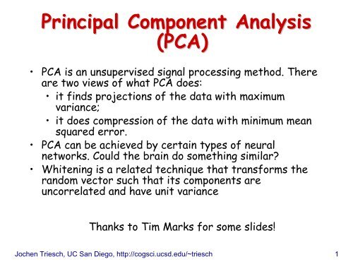
<strong>Principal</strong> <strong>Component</strong> <strong>Analysis</strong><br />
(<strong>PCA</strong>)<br />
• <strong>PCA</strong> is an unsupervised signal processing method. There<br />
are two views of what <strong>PCA</strong> does:<br />
• it finds projections of the data with maximum<br />
variance;<br />
• it does compression of the data with minimum mean<br />
squared error.<br />
• <strong>PCA</strong> can be achieved by certain types of neural<br />
networks. Could the brain do something similar?<br />
• Whitening is a related technique that transforms the<br />
random vector such that its components are<br />
uncorrelated and have unit variance<br />
Thanks to Tim Marks for some slides!<br />
Jochen Triesch, UC San Diego, http://cogsci.ucsd.edu/~triesch 1
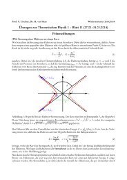
Maximum Variance Projection<br />
• Consider a random vector x with arbitrary joint pdf<br />
• in <strong>PCA</strong> we assume that x has zero mean<br />
• we can always achieve this by constructing x’=x-µ<br />
• Scatter plot and projection y onto a “weight” vector w<br />
w<br />
y<br />
n<br />
T<br />
= w x = ∑<br />
i=<br />
1<br />
cos(<br />
α )<br />
• Motivating question: y is a scalar random variable that<br />
depends on w; for which w is the variance of y maximal?<br />
Jochen Triesch, UC San Diego, http://cogsci.ucsd.edu/~triesch 2<br />
x<br />
y<br />
=<br />
w<br />
×<br />
x<br />
×<br />
w<br />
i<br />
x<br />
i
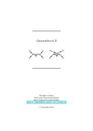
Example:<br />
• consider projecting x onto the red w r and blue w b who<br />
happen to lie along the coordinate axes in this case:<br />
• clearly, the projection<br />
onto w b has the higher<br />
variance, but is there<br />
a w for which it’s even<br />
higher?<br />
Jochen Triesch, UC San Diego, http://cogsci.ucsd.edu/~triesch 3<br />
y<br />
y<br />
r<br />
b<br />
=<br />
=<br />
w<br />
w<br />
T<br />
r<br />
T<br />
b<br />
x<br />
x<br />
=<br />
=<br />
n<br />
∑<br />
i=<br />
1<br />
n<br />
∑<br />
i=<br />
1<br />
w<br />
w<br />
ri<br />
bi<br />
x<br />
i<br />
x<br />
i
• First, what about the mean (expected value) of y?<br />
y<br />
=<br />
w<br />
T<br />
x<br />
=<br />
• so we have:<br />
n<br />
∑<br />
i=<br />
1<br />
n<br />
i=<br />
1<br />
w<br />
i<br />
x<br />
i<br />
E(<br />
y)<br />
= E(<br />
∑ w ) = ∑ ( ) = ∑<br />
ixi<br />
E wi<br />
xi<br />
wiE<br />
( x<br />
i=<br />
1<br />
since x has zero mean, meaning that E(x i ) = 0 for all i.<br />
• This implies that the variance of y is just:<br />
n<br />
• Note that this gets arbitrarily big if w gets longer and<br />
longer, so from now on we restrict w to have length 1,<br />
i.e. (w T w) 1/2 =1<br />
Jochen Triesch, UC San Diego, http://cogsci.ucsd.edu/~triesch 4<br />
n<br />
i=<br />
1<br />
( ( ) ) ) 2<br />
2 ( 2<br />
( ) ( w ) ) T<br />
y − E y = E y E<br />
var( y ) =<br />
E<br />
= x<br />
i<br />
)<br />
=<br />
0
• continuing with some linear algebra tricks:<br />
var(<br />
=<br />
=<br />
E<br />
w<br />
2 ( T 2<br />
y)<br />
= E(<br />
y ) = E ( w x)<br />
)<br />
( T<br />
w x)(<br />
T<br />
x w ) T<br />
w ( T<br />
= E xx )<br />
T<br />
C<br />
x<br />
w<br />
where C x is the correlation matrix (or covariance<br />
matrix) of x.<br />
• We are looking for the vector w that maximizes this<br />
expression<br />
• Linear algebra tells us that the desired vector w is the<br />
eigenvector of C x corresponding to the largest<br />
eigenvalue<br />
Jochen Triesch, UC San Diego, http://cogsci.ucsd.edu/~triesch 5<br />
w
Reminder: Eigenvectors and Eigenvalues<br />
• let A be an nxn (square) matrix. The n-component vector<br />
v is an eigenvector of A with the eigenvalue λ if:<br />
Av = λv<br />
i.e. multiplying v by A only changes the length by a<br />
factor λ but not the orientation.<br />
Example:<br />
• for the scaled identity matrix is every vector is an<br />
eigenvector with identical eigenvalue s<br />
⎛ s<br />
⎜<br />
⎜ M<br />
⎜<br />
⎝0<br />
L<br />
O<br />
L<br />
0⎞<br />
⎟<br />
M ⎟v<br />
= sv<br />
s ⎟<br />
⎠<br />
Jochen Triesch, UC San Diego, http://cogsci.ucsd.edu/~triesch 6
Notes:<br />
• if v is an eigenvector of a matrix A then any scaled<br />
version of v is an Eigenvector of A, too<br />
• if A is a correlation (or covariance) matrix, then all the<br />
eigenvalues are real and nonnegative; the eigenvectors<br />
can be chosen to be mutually orthonormal:<br />
v<br />
T<br />
i<br />
v<br />
k<br />
= δ<br />
ik<br />
⎧1:<br />
i = k<br />
= ⎨<br />
⎩0<br />
: i ≠ k<br />
(δ ik is the so-called Kronecker delta)<br />
• also, if A is a correlation (or covariance) matrix, then A<br />
is positive semidefinite:<br />
T<br />
v Av ≥ 0 ∀ v ≠<br />
Jochen Triesch, UC San Diego, http://cogsci.ucsd.edu/~triesch 7<br />
0
The <strong>PCA</strong> Solution<br />
• The desired direction of maximum variance is the<br />
direction of the unit-length eigenvector v1 of Cx with the<br />
largest eigenvalue<br />
• Next, we want to find the direction whose projection<br />
has the maximum variance among all directions<br />
perpendicular to the first eigenvector v1 . The solution to<br />
this is the unit-length eigenvector v2 of Cx with the 2nd highest eigenvalue.<br />
• In general, the k-th direction whose projection has the<br />
maximum variance among all directions perpendicular to<br />
the first k-1 directions is given by the k-th unit-length<br />
eigenvector of Cx . The eigenvectors are ordered such<br />
that:<br />
λ ≥<br />
1<br />
≥ λ2<br />
≥ Lλn−1<br />
• We say the k-th principal component of x is given by:<br />
y k =<br />
Jochen Triesch, UC San Diego, http://cogsci.ucsd.edu/~triesch 8<br />
v T<br />
k<br />
x<br />
λ<br />
n
What are the variances of the <strong>PCA</strong> projetions?<br />
• From above we have:<br />
( T 2 ) T<br />
( x)<br />
w C w<br />
var( y ) = E =<br />
w x<br />
• Now utilize that w is the k-th eigenvector of C x :<br />
var(<br />
y)<br />
=<br />
=<br />
v<br />
v<br />
T<br />
k<br />
T<br />
k<br />
C<br />
x<br />
v<br />
k<br />
=<br />
( C v )<br />
( ) T<br />
λ k vk<br />
= λk<br />
vk<br />
vk<br />
= k<br />
where in the last step we have exploited that v k has unit<br />
length. Thus, in words, the variance of the k-th principal<br />
component is simply the eigenvalue of the k-th<br />
eigenvector of the correlation/covariance matrix.<br />
Jochen Triesch, UC San Diego, http://cogsci.ucsd.edu/~triesch 9<br />
v<br />
T<br />
k<br />
x<br />
k<br />
λ
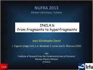
To summarize:<br />
• The eigenvectors v 1 , v 2 , …, v n of the covariance matrix have<br />
corresponding eigenvalues λ 1 ≥ λ 2 ≥ … ≥ λ n . They can be found<br />
with standard algorithms.<br />
• λ 1 is the variance of the projection in the v 1 direction, λ 2 is<br />
the variance of the projection in the v 2 direction, and so on.<br />
• The largest eigenvalue λ 1 corresponds to the principal<br />
component with the greatest variance, the next largest<br />
eigenvalue corresponds to the principal component with the<br />
next greatest variance, etc.<br />
• So, which eigenvector (green or red) corresponds to the<br />
smaller eigenvalue in this example?<br />
Jochen Triesch, UC San Diego, http://cogsci.ucsd.edu/~triesch 10
<strong>PCA</strong> for multinomial Gaussian<br />
• We can think of the joint pdf of the multinomial<br />
Gaussian in terms of the (hyper-) ellipsoidal (hyper-)<br />
surfaces of constant values of the pdf.<br />
• In this setting, principle component analysis (<strong>PCA</strong>) finds<br />
the directions of the axes of the ellipsoid.<br />
• There are two ways to think about what <strong>PCA</strong> does next:<br />
• Projects every point perpendicularly onto the axes of<br />
the ellipsoid.<br />
• Rotates the ellipsoid so its axes are parallel to the<br />
coordinate axes, and translates the ellipsoid so its<br />
center is at the origin.<br />
Jochen Triesch, UC San Diego, http://cogsci.ucsd.edu/~triesch 11
y<br />
Two views of what <strong>PCA</strong> does<br />
a) projects every point x onto the axes of<br />
the ellipsoid to give projection c.<br />
b) rotates space so that the ellipsoid lines up<br />
with the coordinate axes, and translates<br />
space so the ellipsoid’s center is at the<br />
origin.<br />
PC2<br />
c 2<br />
x<br />
c 1<br />
PC1<br />
⎡x⎤<br />
⎢ ⎥<br />
⎣y⎦<br />
Jochen Triesch, UC San Diego, http://cogsci.ucsd.edu/~triesch 12<br />
x<br />
→<br />
c<br />
⎡c<br />
⎢<br />
⎣c<br />
1<br />
2<br />
⎤<br />
⎥<br />
⎦
Transformation matrix for <strong>PCA</strong><br />
• Let V be the matrix whose columns are the eigenvectors<br />
of the covariance matrix, Σ.<br />
• Since the eigenvectors v i are all normalized to have length<br />
1 and are mutually orthogonal, the matrix V is orthonormal<br />
(VV T = I), i.e. it is a rotation matrix<br />
• the inverse rotation transformation is given by the<br />
transpose V T of matrix V<br />
⎡ ↑<br />
⎢<br />
⎢<br />
⎢<br />
⎣ ↓<br />
v 1<br />
↑<br />
v<br />
2<br />
↓<br />
V<br />
L<br />
↑<br />
v<br />
n<br />
↓<br />
⎤<br />
⎥<br />
⎥<br />
⎥<br />
⎦<br />
⎡←<br />
⎢<br />
⎢<br />
←<br />
⎢<br />
⎢<br />
⎣←<br />
→⎤<br />
→<br />
⎥<br />
⎥<br />
⎥<br />
⎥<br />
→⎦<br />
Jochen Triesch, UC San Diego, http://cogsci.ucsd.edu/~triesch 13<br />
V<br />
v1 v<br />
M<br />
v<br />
2<br />
n<br />
T
Transformation matrix for <strong>PCA</strong><br />
• <strong>PCA</strong> transforms the point x (original coordinates) into the<br />
point c (new coordinates) by subtracting the mean from x<br />
(z = x – m) and multiplying the result by V T<br />
⎡←<br />
⎢<br />
⎢<br />
←<br />
⎢<br />
⎢<br />
⎣←<br />
V<br />
v1<br />
v2<br />
M<br />
v<br />
n<br />
T<br />
→⎤<br />
→<br />
⎥<br />
⎥<br />
⎥<br />
⎥<br />
→⎦<br />
⎡↑⎤<br />
⎢ ⎥<br />
⎢z<br />
⎥<br />
⎢ ⎥<br />
⎣↓⎦<br />
• this is a rotation because V T is an orthonormal matrix<br />
• this is a projection of z onto PC axes, because v 1 • z is<br />
projection of z onto PC1 axis, v 2 • z is projection onto PC2<br />
axis, etc.<br />
z<br />
Jochen Triesch, UC San Diego, http://cogsci.ucsd.edu/~triesch 14<br />
=<br />
⎡v<br />
⎢<br />
⎢<br />
v<br />
⎢<br />
⎢<br />
⎣v<br />
1<br />
2<br />
n<br />
c<br />
M<br />
⋅<br />
⋅<br />
⋅<br />
z⎤<br />
z<br />
⎥<br />
⎥<br />
⎥<br />
⎥<br />
z⎦
• <strong>PCA</strong> expresses the mean-subtracted point, z = x – m, as a<br />
weighted sum of the eigenvectors vi . To see this, start<br />
with:<br />
T<br />
⎡←<br />
⎢<br />
⎢<br />
←<br />
⎢<br />
⎢<br />
⎣←<br />
V<br />
v<br />
v<br />
1<br />
2<br />
M<br />
v<br />
D<br />
→⎤<br />
→<br />
⎥<br />
⎥<br />
⎥<br />
⎥<br />
→⎦<br />
• multiply both sides of the equation from the left by V:<br />
VV T z = Vc | exploit that V is orthonormal<br />
z = Vc | i.e. we can easily reconstruct z from c<br />
z<br />
⎡↑⎤<br />
⎢ ⎥<br />
⎢z<br />
⎥<br />
⎢ ⎥<br />
⎣↓⎦<br />
=<br />
=<br />
⎡ ↑<br />
⎢<br />
⎢v<br />
⎢<br />
⎣ ↓<br />
1<br />
↑<br />
v<br />
2<br />
↓<br />
V<br />
c<br />
⎡c1<br />
⎤<br />
↑ ⎤ ⎢ ⎥<br />
⎥ ⎢<br />
c2<br />
v ⎥<br />
n ⎥ ⎢ M ⎥<br />
↓ ⎥<br />
⎦ ⎢ ⎥<br />
⎣cn<br />
⎦<br />
Jochen Triesch, UC San Diego, http://cogsci.ucsd.edu/~triesch 15<br />
z<br />
⎡↑⎤<br />
⎢ ⎥<br />
⎢z<br />
⎥<br />
⎢ ⎥<br />
⎣↓⎦<br />
=<br />
c<br />
=<br />
⎡ ↑ ⎤<br />
⎢ ⎥<br />
⎢v1<br />
⎥<br />
⎢ ⎥<br />
⎣ ↓ ⎦<br />
c<br />
⎡ c<br />
⎢<br />
⎢<br />
c<br />
⎢ M<br />
⎢<br />
⎣c<br />
+<br />
1<br />
2<br />
D<br />
⎤<br />
⎥<br />
⎥<br />
⎥<br />
⎥<br />
⎦<br />
c<br />
⎡ ↑<br />
⎢<br />
⎢v<br />
⎢<br />
⎣ ↓<br />
L 1<br />
2 2<br />
⎤<br />
⎥<br />
⎥<br />
⎥<br />
⎦<br />
+<br />
L<br />
+<br />
c<br />
n<br />
⎡ ↑<br />
⎢<br />
⎢v<br />
⎢<br />
⎣ ↓<br />
n<br />
⎤<br />
⎥<br />
⎥<br />
⎥<br />
⎦
<strong>PCA</strong> for data compression<br />
What if you wanted to transmit someone’s height and weight,<br />
but you could only give a single number?<br />
• Could give only height, x<br />
— = (uncertainty when height is known)<br />
• Could give only weight, y<br />
— = (uncertainty when weight is known)<br />
• Could give only c 1 ,<br />
the value of first PC<br />
— = (uncertainty when first PC is known)<br />
• Giving the first PC minimizes<br />
the squared error of the result.<br />
weight<br />
Jochen Triesch, UC San Diego, http://cogsci.ucsd.edu/~triesch 16<br />
y<br />
PC2<br />
To compress n-dimensional data into k dimensions, order the<br />
principal components in order of largest-to-smallest<br />
eigenvalue, and only save the first k components.<br />
c 2<br />
x<br />
c 1<br />
PC1<br />
height
• Equivalent view: To compress n-dimensional data into k
<strong>PCA</strong> vs. Discrimination<br />
• variance maximization or compression are different from<br />
discrimination!<br />
• consider this data coming stemming from two classes?<br />
• which direction has max. variance, which discriminates<br />
between the two clusters?<br />
Jochen Triesch, UC San Diego, http://cogsci.ucsd.edu/~triesch 18
Application: <strong>PCA</strong> on face images<br />
• 120 × 100 pixel grayscale 2D images of faces. Each<br />
image is considered to be a single point in face space (a<br />
single sample from a random vector):<br />
⎡↑⎤<br />
⎢ ⎥<br />
⎢x⎥<br />
⎢ ⎥<br />
⎣↓⎦<br />
• How many dimensions is the vector x ?<br />
n = 120 • 100 = 12000<br />
• Each dimension (each pixel) can take values between 0<br />
and 255 (8 bit grey scale images).<br />
• You can easily visualize points in this 12000 dimensional<br />
space!<br />
Jochen Triesch, UC San Diego, http://cogsci.ucsd.edu/~triesch 19
The original images (12 out of 97)<br />
Jochen Triesch, UC San Diego, http://cogsci.ucsd.edu/~triesch 20
The mean face<br />
Jochen Triesch, UC San Diego, http://cogsci.ucsd.edu/~triesch 21
• Let x 1 , x 2 , …, x p be the p sample images (n-dimensional).<br />
• Find the mean image, m, and subtract it from each<br />
image: z i = x i – m<br />
• Let A be the matrix whose columns are the<br />
mean-subtracted sample images.<br />
⎡ ↑ ↑ ↑ ⎤<br />
⎢<br />
⎥<br />
A = ⎢z1<br />
z 2 L z p ⎥ n ×<br />
⎢<br />
⎥<br />
⎣ ↓ ↓ ↓ ⎦<br />
• Estimate the covariance matrix:<br />
Σ<br />
=<br />
1<br />
Cov( A)<br />
= A A<br />
p −1<br />
What are the dimensions of Σ ?<br />
matrix<br />
Jochen Triesch, UC San Diego, http://cogsci.ucsd.edu/~triesch 22<br />
T<br />
p
The transpose trick<br />
The eigenvectors of Σ are the principal component directions.<br />
Problem:<br />
• Σ is a nxn (12000×12000) matrix. It’s too big for us to<br />
find its eigenvectors numerically. In addition, only the<br />
first p eigenvalues are useful; the rest will all be zero,<br />
because we only have p samples.<br />
Solution: Use the following trick.<br />
• Eigenvectors of Σ are eigenvectors of AA T ; but instead<br />
of eigenvectors of AA T , the eigenvectors of A T A are easy<br />
to find<br />
What are the dimensions of A T A ? It’s a p×p matrix: it’s easy<br />
to find eigenvectors since p is relatively small.<br />
Jochen Triesch, UC San Diego, http://cogsci.ucsd.edu/~triesch 23
• We want the eigenvectors of AA T , but instead we calculated<br />
the eigenvectors of A T A. Now what?<br />
• Let v i be an eigenvector of A T A, whose eigenvalue is λ i<br />
(ATA)vi = ? λivi A (ATAv ) i = A(λivi) AAT (Av ) i = λi (Avi) • Thus if v i is an eigenvector of A T A ,<br />
Av i is an eigenvector of AA T , with the same eigenvalue.<br />
Av 1 , Av 2 , … , Av n are the eigenvectors of Σ.<br />
u 1 = Av 1 , u 2 = Av 2 , …, u n = Av n are called eigenfaces.<br />
Jochen Triesch, UC San Diego, http://cogsci.ucsd.edu/~triesch 24
Eigenfaces<br />
• Eigenfaces (the principal component directions of face<br />
space) provide a low-dimensional representation of any<br />
face, which can be used for:<br />
• Face image compression and reconstruction<br />
• Face recognition<br />
• Facial expression recognition<br />
Jochen Triesch, UC San Diego, http://cogsci.ucsd.edu/~triesch 25
The first 8 eigenfaces<br />
Jochen Triesch, UC San Diego, http://cogsci.ucsd.edu/~triesch 26
<strong>PCA</strong> for low-dimensional low dimensional face<br />
representation<br />
• To approximate a face using only k dimensions, order the<br />
eigenfaces in order of largest-to-smallest eigenvalue,<br />
and only use the first k eigenfaces.<br />
z<br />
⎡↑⎤<br />
⎢ ⎥<br />
⎢z<br />
⎥<br />
⎢ ⎥<br />
⎣↓⎦<br />
=<br />
=<br />
⎡ ↑<br />
⎢<br />
⎢u1<br />
⎢<br />
⎣ ↓<br />
⎡←<br />
⎢<br />
⎢←<br />
⎢<br />
⎣←<br />
U<br />
u<br />
u<br />
u<br />
1<br />
2<br />
M<br />
k<br />
T<br />
→⎤<br />
⎥<br />
→⎥<br />
⎥<br />
→⎦<br />
U c<br />
↑<br />
u2<br />
↓<br />
L<br />
⎡c1<br />
⎤<br />
↑ ⎤ ⎢ ⎥<br />
⎥ ⎢<br />
c2<br />
u ⎥<br />
k ⎥ ⎢ M ⎥<br />
↓ ⎥<br />
⎦ ⎢ ⎥<br />
⎣ck<br />
⎦<br />
⎡ ↑ ⎤ ⎡ ↑ ⎤<br />
⎢ ⎥ ⎢ ⎥<br />
= c1<br />
⎢u1<br />
⎥ + c2<br />
⎢u2<br />
⎥ + L<br />
⎢ ⎥ ⎢ ⎥<br />
⎣ ↓ ⎦ ⎣ ↓ ⎦<br />
⎡ ↑ ⎤<br />
⎢ ⎥<br />
⎢uk<br />
⎥<br />
⎢ ⎥<br />
⎣ ↓ ⎦<br />
Jochen Triesch, UC San Diego, http://cogsci.ucsd.edu/~triesch 27<br />
⎡↑⎤<br />
⎢ ⎥<br />
⎢z<br />
⎥<br />
⎢ ⎥<br />
⎣↓⎦<br />
• <strong>PCA</strong> approximates a mean-subtracted face, z = x – m, as<br />
a weighted sum of the first k eigenfaces:<br />
z<br />
=<br />
c<br />
⎡c<br />
⎢<br />
⎢c<br />
M ⎢<br />
⎣c<br />
1<br />
2<br />
k<br />
⎤<br />
⎥<br />
⎥<br />
⎥<br />
⎦<br />
+<br />
c<br />
k
• To approximate the actual face we have to add the mean<br />
face m to the reconstruction of z:<br />
x<br />
=<br />
= U c + m<br />
=<br />
=<br />
z + m<br />
⎡ ↑<br />
⎢<br />
⎢u1<br />
⎢<br />
⎣ ↓<br />
c<br />
1<br />
↑<br />
u<br />
2<br />
↓<br />
⎡ ↑ ⎤<br />
⎢ ⎥<br />
⎢u1<br />
⎥ +<br />
⎢ ⎥<br />
⎣ ↓ ⎦<br />
⎡c1<br />
⎤<br />
↑ ⎤ ⎢ ⎥ ⎡↑<br />
⎤<br />
⎥ ⎢<br />
c2<br />
⎢ ⎥<br />
L u ⎥<br />
k ⎥ + ⎢m<br />
⎢ M ⎥ ⎥<br />
↓ ⎥ ⎢ ⎥<br />
⎦ ⎢ ⎥ ⎣↓<br />
⎦<br />
⎣ck<br />
⎦<br />
⎡ ↑ ⎤ ⎡ ↑ ⎤ ⎡↑<br />
⎤<br />
⎢ ⎥ ⎢ ⎥ ⎢ ⎥<br />
c2<br />
⎢u<br />
2 ⎥ + L + ck<br />
⎢u<br />
k ⎥ + ⎢m⎥<br />
⎢ ⎥ ⎢ ⎥ ⎢ ⎥<br />
⎣ ↓ ⎦ ⎣ ↓ ⎦ ⎣↓<br />
⎦<br />
• The reconstructed face is simply the mean face with<br />
some fraction of each eigenface added to it<br />
Jochen Triesch, UC San Diego, http://cogsci.ucsd.edu/~triesch 28
The mean face<br />
Jochen Triesch, UC San Diego, http://cogsci.ucsd.edu/~triesch 29
Approximating a face using the<br />
first 10 eigenfaces<br />
Jochen Triesch, UC San Diego, http://cogsci.ucsd.edu/~triesch 30
Approximating a face using the<br />
first 20 eigenfaces<br />
Jochen Triesch, UC San Diego, http://cogsci.ucsd.edu/~triesch 31
Approximating a face using the<br />
first 40 eigenfaces<br />
Jochen Triesch, UC San Diego, http://cogsci.ucsd.edu/~triesch 32
Approximating a face using all<br />
97 eigenfaces<br />
Jochen Triesch, UC San Diego, http://cogsci.ucsd.edu/~triesch 33
Notes:<br />
• not surprisingly, the approximation of the reconstructed<br />
faces get better when more eigenfaces are used<br />
• In the extreme case of using no eigenface at all, the<br />
reconstruction of any face image is just the average<br />
face<br />
• In the other extreme of using all 97 eigenfaces, the<br />
reconstruction is exact, since the image was in the<br />
original training set of 97 images. For a new face image,<br />
however, its reconstruction based on the 97 eigenfaces<br />
will only approximately match the original.<br />
• What regularities does each eigenface capture? See<br />
movie.<br />
Jochen Triesch, UC San Diego, http://cogsci.ucsd.edu/~triesch 34
Eigenfaces in 3D<br />
• Blanz and Vetter (SIGGRAPH ’99). The video can be<br />
found at:<br />
http://graphics.informatik.uni-freiburg.de/Sigg99.html<br />
Jochen Triesch, UC San Diego, http://cogsci.ucsd.edu/~triesch 35