Improved DAG SVM: A New Method for Multi-Class SVM Classification
Improved DAG SVM: A New Method for Multi-Class SVM Classification
Improved DAG SVM: A New Method for Multi-Class SVM Classification
You also want an ePaper? Increase the reach of your titles
YUMPU automatically turns print PDFs into web optimized ePapers that Google loves.
548<br />
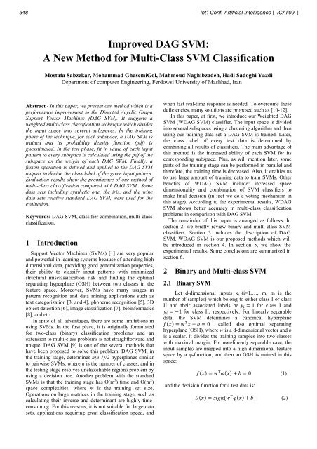
<strong>Improved</strong> <strong>DAG</strong> <strong>SVM</strong>:<br />
A <strong>New</strong> <strong>Method</strong> <strong>for</strong> <strong>Multi</strong>-<strong>Class</strong> <strong>SVM</strong> <strong>Class</strong>ification<br />
Mostafa Sabzekar, Mohammad GhasemiGol, Mahmoud Naghibzadeh, Hadi Sadoghi Yazdi<br />
Department of computer Engineering, Ferdowsi University of Mashhad, Iran<br />
Abstract - In this paper, we present our method which is a<br />
per<strong>for</strong>mance improvement to the Directed Acyclic Graph<br />
Support Vector Machines (<strong>DAG</strong> <strong>SVM</strong>). It suggests a<br />
weighted multi-class classification technique which divides<br />
the input space into several subspaces. In the training<br />
phase of the technique, <strong>for</strong> each subspace, a <strong>DAG</strong> <strong>SVM</strong> is<br />
trained and its probability density function (pdf) is<br />
guesstimated. In the test phase, fit in value of each input<br />
pattern to every subspace is calculated using the pdf of the<br />
subspace as the weight of each <strong>DAG</strong> <strong>SVM</strong>. Finally, a<br />
fusion operation is defined and applied to the <strong>DAG</strong> <strong>SVM</strong><br />
outputs to decide the class label of the given input pattern.<br />
Evaluation results show the prominence of our method of<br />
multi-class classification compared with <strong>DAG</strong> <strong>SVM</strong>. Some<br />
data sets including synthetic one, the iris, and the wine<br />
data sets relative standard <strong>DAG</strong> <strong>SVM</strong>, were used <strong>for</strong> the<br />
evaluation.<br />
Keywords: <strong>DAG</strong> <strong>SVM</strong>, classifier combination, multi-class<br />
classification.<br />
1 Introduction<br />
Support Vector Machines (<strong>SVM</strong>s) [1] are very popular<br />
and powerful in learning systems because of attending high<br />
dimensional data, providing good generalization properties,<br />
their ability to classify input patterns with minimized<br />
structural misclassification risk and finding the optimal<br />
separating hyperplane (OSH) between two classes in the<br />
feature space. Moreover, <strong>SVM</strong>s have many usages in<br />
pattern recognition and data mining applications such as<br />
text categorization [3, and 4], phoneme recognition [5], 3D<br />
object detection [6], image classification [7], bioin<strong>for</strong>matics<br />
[8], and etc.<br />
In spite of all advantages, there are some limitations in<br />
using <strong>SVM</strong>s. In the first place, it is originally <strong>for</strong>mulated<br />
<strong>for</strong> two-class (binary) classification problems and an<br />
extension to multi-class problems is not straight<strong>for</strong>ward and<br />
unique. <strong>DAG</strong> <strong>SVM</strong> [9] is one of the several methods that<br />
have been proposed to solve this problem. <strong>DAG</strong> <strong>SVM</strong>, in<br />
the training stage, determines n(n-1)/2 hyperplanes similar<br />
to pairwise <strong>SVM</strong>s, where n is the number of classes, and in<br />
the testing stage resolves unclassifiable regions problem by<br />
using a decision tree. Another problem with the standard<br />
<strong>SVM</strong>s is that the training stage has O(m 3 ) time and O(m 2 )<br />
space complexities, where m is the training set size.<br />
Operations on large matrices in the training stage, such as<br />
calculating their inverse and determinant are highly timeconsuming.<br />
For this reasons, it is not suitable <strong>for</strong> large data<br />
sets, applications requiring great classification speed, and<br />
when fast real-time response is needed. To overcome these<br />
deficiencies, many solutions are proposed such as [10-12].<br />
In this paper, at first, we introduce our Weighted <strong>DAG</strong><br />
<strong>SVM</strong> (W<strong>DAG</strong> <strong>SVM</strong>) classifier. The input space is divided<br />
into several subspaces using a clustering algorithm and then<br />
using our training data set a <strong>DAG</strong> <strong>SVM</strong> is trained. Later,<br />
the class label of every test data is determined by<br />
combining all results of classifiers. The main advantage of<br />
this method is the increased ability of each <strong>SVM</strong> <strong>for</strong> its<br />
corresponding subspace. Plus, as will mention later, some<br />
parts of the training stage can be per<strong>for</strong>med in parallel and<br />
there<strong>for</strong>e, the training time is decreased. Also, it enables us<br />
to use large amount of training data to train <strong>SVM</strong>s. Other<br />
benefits of W<strong>DAG</strong> <strong>SVM</strong> include: increased space<br />
dimensionality and combination of <strong>SVM</strong> classifiers to<br />
make final decision (in fact we do a voting mechanism in<br />
this stage). According to the experimental results, W<strong>DAG</strong><br />
<strong>SVM</strong> shows better accuracy in multi-class classification<br />
problems in comparison with <strong>DAG</strong> <strong>SVM</strong>.<br />
The remainder of this paper is arranged as follows. In<br />
section 2, we briefly review binary and multi-class <strong>SVM</strong><br />
classifiers. Section 3 includes the description of <strong>DAG</strong><br />
<strong>SVM</strong>. W<strong>DAG</strong> <strong>SVM</strong> is our proposed methods which will<br />
be introduced in section 4. In section 5, we show the<br />
experimental results. Some conclusions are summarized in<br />
section 6.<br />
2 Binary and <strong>Multi</strong>-class <strong>SVM</strong><br />
2.1 Binary <strong>SVM</strong><br />
Int'l Conf. Artificial Intelligence | ICAI'09 |<br />
Let d-dimensional inputs xi (i=1,…, m, m is the<br />
number of samples) which belong to either class I or class<br />
II and their associated labels be � � �� <strong>for</strong> class I and<br />
� � ��� <strong>for</strong> class II, respectively. For linearly separable<br />
data, the <strong>SVM</strong> determines a canonical hyperplane<br />
���� �� � ����� , called also optimal separating<br />
hyperplane (OSH), where w is a d-dimensional vector and b<br />
is a scalar. It divides the training samples into two classes<br />
with maximal margin. For non-linearly separable case, the<br />
input samples are mapped into a high-dimensional feature<br />
space by a �-function, and then an OSH is trained in this<br />
space:<br />
������� �� � ���� ���� (1)<br />
and the decision function <strong>for</strong> a test data is:<br />
���� ������� � ���� �� (2)
Int'l Conf. Artificial Intelligence | ICAI'09 | 549<br />
Considering the noise with slack variables �� and error<br />
�<br />
penalty term ��� ���� �� , the optimal hyperplane can be<br />
found by solving the following quadratic optimization<br />
problem:<br />
����� �<br />
� ����� �<br />
������� ���<br />
��� ���������� ���� ���� ����� (3)<br />
2.2 <strong>Multi</strong>-class <strong>SVM</strong><br />
<strong>SVM</strong> <strong>for</strong>mulation has been originally developed <strong>for</strong><br />
binary classification problems and finding the direct<br />
<strong>for</strong>mulation <strong>for</strong> multi-class case is not easy and still an ongoing<br />
research issue. In two ways we can have a multi-class<br />
<strong>SVM</strong> classifier; one is to directly consider all data in one<br />
optimization <strong>for</strong>mulation, and the other is to decompose<br />
multi-class problem to several binary problems. The second<br />
solution is a better idea and has been considered more than<br />
the first approach [13-17] because binary classifiers are<br />
easier to implement and moreover some powerful<br />
algorithms such as Support Vector Machine (<strong>SVM</strong>) are<br />
inherently binary [18]. Two major decomposition<br />
implementations are: “one-against-all” and “one-against<br />
one”.<br />
The one-against-all [1] method constructs n <strong>SVM</strong>s<br />
where n is the number of classes. The i th <strong>SVM</strong> is trained to<br />
separate the i th class from remaining classes. The oneagainst-one<br />
[14] (pairwise <strong>SVM</strong>s) instead, constructs n(n-<br />
1)/2 decision functions <strong>for</strong> all the combinations of class<br />
pairs. In determination of a decision function <strong>for</strong> a class<br />
pair, we use the training data <strong>for</strong> the corresponding two<br />
classes. Thus, in each training session, the number of the<br />
training data is reduced considerably compared to oneagainst-all<br />
support vector machines, which use all the<br />
training data. Experimental results in [19] indicate that the<br />
one-against-one is more suitable <strong>for</strong> practical use. We<br />
continue our discussion with focus on the pairwise <strong>SVM</strong>s<br />
method in next section (more details appeared in [20]).<br />
3 <strong>DAG</strong> <strong>SVM</strong><br />
A problem with both on-against-all and pairwise support<br />
vector machines is unclassifiable regions. In pairwise<br />
<strong>SVM</strong>s, let the decision function <strong>for</strong> class i against class j,<br />
with the maximal margin, be:<br />
� ����� �� �� � ���� �������������������������������������<br />
where � �� is the d-dimensional vector, ���� is a mapping<br />
function that maps � into the d-dimensional feature space,<br />
� ���is the bias term, and �� ����� ��� �����.<br />
The regions Ri are shown in Figure 1 with labels of class I,<br />
II, and III.<br />
� � ����� ����� � �� � � ���� � � �� � � ���������������������<br />
If � is in Ri, we classify � into class i. If � is not in<br />
� ��� � ���� � � ��, � is classified by voting. Namely, <strong>for</strong> the<br />
input vector �� � �����is calculated at follow:<br />
where<br />
�<br />
����� � � ������������ ��������������������������<br />
�������<br />
�������������� � ��<br />
������� ��<br />
��������������� � �� �������������������������<br />
and x is classified into class:<br />
��� ���<br />
���������� � ������������������������������������������<br />
If ����� �,� ���� ���� and� ���� � � � �������� � ��Thus,<br />
� is classified into �. But if any of � ���� is not ���, ���<br />
may be satisfied <strong>for</strong> plural is. In this case, � is<br />
unclassifiable. In the shaded region in Figure 1,<br />
� ���� ����� ����������� . There<strong>for</strong>e, this region is<br />
unclassifiable, although the unclassifiable region is much<br />
smaller than that <strong>for</strong> the one-against-all support vector<br />
machine.<br />
Figure 1: Unclassifiable regions by the pairwise <strong>for</strong>mulation.<br />
In pairwise <strong>SVM</strong>s, classification reduces the<br />
unclassifiable regions that occur <strong>for</strong> one-against-all<br />
support vector machines but it still exists. To resolve this<br />
problem, Vapnik [2] proposed to use continuous decision<br />
functions. Namely, we classify a datum into the class with<br />
maximum value of the decision functions. Inoue and Abe<br />
[21] proposed fuzzy support vector machines, in which<br />
membership functions are defined using the decision<br />
functions. Another popular solution is <strong>DAG</strong> <strong>SVM</strong> that uses<br />
a decision tree in the testing stage. Training of a <strong>DAG</strong> is<br />
the same as conventional pairwise <strong>SVM</strong>s. <strong>Class</strong>ification by<br />
<strong>DAG</strong>s is faster than by conventional pairwise <strong>SVM</strong>s or<br />
pairwise fuzzy <strong>SVM</strong>s. Figure 2 shows the decision tree <strong>for</strong><br />
the three classes shown in Figure 1. In the figure, � shows<br />
that x does not belong to class i. As the top-level<br />
classification, we can choose any pair of classes. And<br />
except <strong>for</strong> the leaf node if � ����� ��, we consider that x<br />
does not belong to class j, and if � ����� �� not class i.<br />
Thus, if � ����� ��, x does not belong to class II.<br />
There<strong>for</strong>e, it belongs to either class I or class III, and the<br />
next classification pair is classes I and III.
550 Int'l Conf. Artificial Intelligence | ICAI'09 |<br />
Figure 2: <strong>DAG</strong> classification.<br />
The generalization regions become as shown in Figure 3.<br />
Unclassifiable regions are resolved, but clearly the<br />
generalization regions depend on the tree <strong>for</strong>mation.<br />
Figure 3: Generalization region by <strong>DAG</strong> classification.<br />
4 The Proposed <strong>Method</strong><br />
In this section we propose W<strong>DAG</strong> <strong>SVM</strong>. Suppose that<br />
we have a large group of data with different class labels<br />
that are completely mixed together. Usual methods <strong>for</strong> this<br />
multi-class classification problem such as one-against-all<br />
or <strong>DAG</strong> face some difficulties:<br />
� The kernel matrices that are constructed in the<br />
training stage are large and computations on such<br />
matrices, <strong>for</strong> example finding their inverse and<br />
determinant, consume tremendous CPU time and<br />
takes lots of space.<br />
� The accuracy of classification is low especially<br />
when the classes mixed.<br />
W<strong>DAG</strong> <strong>SVM</strong> attempts to overcome these limitations by<br />
dividing the input space into several subspaces and train a<br />
<strong>DAG</strong> <strong>SVM</strong> <strong>for</strong> each of them.<br />
Figure 4 shows the idea of W<strong>DAG</strong> <strong>SVM</strong> abstractly.<br />
Firstly, we see all training data that are clustered into three<br />
regions (the regions are colored red, green, and blue if the<br />
paper is printed in color). In each region, a <strong>DAG</strong> <strong>SVM</strong> is<br />
trained but the pdf (probability density function) of each<br />
cluster specifies the significance of each <strong>DAG</strong> <strong>SVM</strong>. For<br />
each cluster, this important degree is large in the middle<br />
but decreases in the periphery, which is shown with<br />
blurred color in peripheries. Figure 5 shows details and<br />
following sub-sections explain the proposed approach with<br />
more details.<br />
Figure 4: The overall view of W<strong>DAG</strong> <strong>SVM</strong> with 3 clusters in 2-D<br />
spaces.<br />
Description of Training Module<br />
The training stage (Figure 5.a) consists of three levels. In<br />
the first level, the training data is divided into N clusters by<br />
K-Means algorithm. Then the statistical parameters of each<br />
cluster <strong>for</strong> normal pdf are extracted. These parameters<br />
include covariance and mean vectors which are defined as<br />
follows:<br />
Suppose that � � � �� ��� ����� ��� � and � � �<br />
�� ��� ����� �� � are vectors in � � space. Also, � � �<br />
�� ��� ����� �� and � � � �� ��� ����� �� are i th sample<br />
�� � ���� � � �� in � � . There<strong>for</strong>e:<br />
� �<br />
� �� �<br />
�<br />
���� � � �<br />
� ��������������������������������������������� �<br />
���<br />
�<br />
��� ���� �������� � � ������ � ���������������������<br />
���<br />
where ���� �� is the mean vector with d members,<br />
and������ is the covariance matrix (d×d), where d is the<br />
�<br />
number of features <strong>for</strong> the input data. Theses parameters<br />
are used to assign a Gaussian distribution function (12) to<br />
each cluster that is used <strong>for</strong> weighting procedure in the<br />
testing stage:<br />
���� � �<br />
�<br />
�������<br />
������������ �� ��������������������<br />
where ������ �� �� are the mean vector and the covariance<br />
matrix of the M th cluster. These Gaussians can overlap<br />
which enables us to make a fuzzy boundary between<br />
clusters. Finally, in each cluster, existent data is trained<br />
using <strong>DAG</strong> <strong>SVM</strong> in the third level. Training of <strong>DAG</strong> <strong>SVM</strong><br />
is similar to one-against-one <strong>SVM</strong>s.<br />
The outputs of the training stage are a Gaussian<br />
distribution function and optimal decision hyperplanes of<br />
each cluster that are used in the testing stage. Note that we<br />
assumed that the samples are not independent and have use<br />
covariance matrix to obtain a more accurate distribution<br />
function <strong>for</strong> the representation of each cluster.
Int'l Conf. Artificial Intelligence | ICAI'09 | 551<br />
(b)<br />
(a)<br />
Figure 5: General overview of the proposed W<strong>DAG</strong> <strong>SVM</strong><br />
scheme, (a) training module and (b) testing module.<br />
Description of Testing Module<br />
Testing module includes basic levels such as weighing<br />
procedure (WP), decision making, and voting which are<br />
shown in Figure 5.b and discussed separately as follows:<br />
Level 1: Weighting Procedure (WP)<br />
In this level, the membership degree of each testing data<br />
to each cluster is calculated using Gaussian distribution<br />
functions which have been achieved in the previous section.<br />
Let �� � �<br />
����� �� �be a set of -dimensional test samples.<br />
Membership degree of �� in relation to Mth cluster<br />
�� � ���� � � �� according to (12) is given as:<br />
� � � �<br />
�<br />
�������<br />
������� � ����� �� �� � ������������������<br />
Note that the output of the weighting procedure is � �<br />
where M=1,..,N and N is the number of clusters.<br />
Level 2: Decision Making<br />
The label of � � (where � � is a test data) is calculated using<br />
majority-based decision obtained from <strong>DAG</strong> <strong>SVM</strong> which is<br />
trained <strong>for</strong> the M th cluster.<br />
Let the decision function <strong>for</strong> class i against class j, <strong>for</strong> the<br />
M th cluster with the maximal margin, be:<br />
� �� � ���� �� �� � ���� �� ��������������������������������<br />
and in each cluster we follow the corresponding <strong>DAG</strong> <strong>SVM</strong><br />
structure <strong>for</strong> determining class label of � �. At the end of this<br />
stage, each cluster returns a local class label � � (i=1, ..., N),<br />
where N is the number of clusters. Voting is the final stage<br />
that determines the global class label of � � considering<br />
clusters judgment and membership degrees.<br />
Level 3: Voting<br />
Output of this level is achieved by the fusion operation.<br />
The combining procedure can improve classification rate.<br />
Suppose that � ��� ��� ����� �� is set of labels <strong>for</strong> a given<br />
test sample � � that are determined by N <strong>DAG</strong> <strong>SVM</strong>, also<br />
���� ��� ����� �� is set of membership degrees of a<br />
same test sample � � to each cluster, where N is the number<br />
of clusters. Finally, output is achieved by:<br />
where<br />
and<br />
����������� � ��� �������������������������������� ������<br />
�� ��������������������������������������������� ��� ��<br />
� � � ���� � � ������ � � �� � � �������������������������<br />
where n is the number of classes. � � is set of labels which<br />
mention to class i and � � is sum of their weights. Equation<br />
(15) demonstrate that � � is assigned to a class with<br />
maximum � �. In the other words, two following points are<br />
required to classification of input samples:<br />
� Number of labels assigned to each class<br />
� Weight (degree of importance that is achieved<br />
from WP) of each classifier that participates in<br />
voting procedure.<br />
There<strong>for</strong>e, if a class is mentioned with a large number of<br />
<strong>DAG</strong> <strong>SVM</strong> and also weights of these classifiers be high<br />
enough, then the test sample is assigned to it.<br />
5 Experimental Evaluation<br />
The proposed method has been evaluated over a series of<br />
synthetic data. In Table 1, the accuracy of <strong>DAG</strong> <strong>SVM</strong> and<br />
W<strong>DAG</strong> <strong>SVM</strong> classifiers <strong>for</strong> a series of synthetic data has<br />
been compared. The number of synthetic data is 150 (50<br />
data in each class). Four types of data are considered. In<br />
data type 1, separate data is used and gradually in data set 2<br />
to 4 classes are interlaced (shown in Figure 6). As shown in<br />
Table 1, comparing the two methods, W<strong>DAG</strong> <strong>SVM</strong> gives<br />
better results in each level of interlacing.
552 Int'l Conf. Artificial Intelligence | ICAI'09 |<br />
The power of our method is apparent especially when the<br />
data are completely mixed. Also our proposed method is<br />
evaluated <strong>for</strong> iris and wine data sets and its results are<br />
summarized in Table 2. According to Table 2 it can be seen<br />
that the accuracy of W<strong>DAG</strong> <strong>SVM</strong> classifier <strong>for</strong> both noisy<br />
and without noise iris data set and also wine data set is<br />
more than the <strong>DAG</strong> <strong>SVM</strong>.<br />
It is mentionable that choosing the number of clusters is a<br />
trade-off. This value must be chosen in a way that in each<br />
cluster, there are data points from whole of the classes. We<br />
tested different values <strong>for</strong> N (the number of clusters) in our<br />
experiments and we found constant recognition rate <strong>for</strong><br />
N=3 and greater.<br />
We also claim that our method is more efficient in<br />
execution time. Table 3 shows the learning stage times <strong>for</strong><br />
synthesize, iris, and wine data sets. The number of data<br />
points in Data 1 data set is 1500 (500 data points <strong>for</strong> each<br />
class) and in Data 2 data set is 6000 (2000 data points <strong>for</strong><br />
each class).<br />
Table 1: Experimental results of <strong>DAG</strong> <strong>SVM</strong> and W<strong>DAG</strong> <strong>SVM</strong> in<br />
2-dimensional spaces (N=3)<br />
Number of<br />
testing data<br />
40 sample of<br />
Data1<br />
40 sample of<br />
Data2<br />
40 sample of<br />
Data3<br />
40 sample of<br />
Data4<br />
Recognition<br />
rate of<br />
<strong>DAG</strong> <strong>SVM</strong><br />
Recognition<br />
rate of<br />
W<strong>DAG</strong> <strong>SVM</strong><br />
100 100<br />
96 100<br />
96 100<br />
69 98<br />
Figure 6: Synthetic data <strong>for</strong> experiment<br />
6 Conclusion<br />
In this paper, we proposed a weighted <strong>DAG</strong> support<br />
vector machine algorithm <strong>for</strong> multi-class classification<br />
problems. The important contributions of the proposed<br />
algorithm can be summarized as follows:<br />
� Dividing input space to subspaces (space<br />
linearization)<br />
� Applying multi expert system instead of one<br />
classifier<br />
� Using the power of classifier fusion in the mixing<br />
results<br />
After dividing of samples using the clustering algorithm,<br />
<strong>for</strong> each part a <strong>DAG</strong> <strong>SVM</strong> is trained and weighting<br />
procedure helps to fusion multi-trained <strong>SVM</strong>s. Captured<br />
results over synthetic sample dataset showed mixed data<br />
could be classified with high precisions. The outcome<br />
recommends applying the W<strong>DAG</strong> <strong>SVM</strong> (the proposed<br />
method) to low signal to noise ratio environment and fused<br />
samples. Also we applied the W<strong>DAG</strong> <strong>SVM</strong> to the standard<br />
iris and wine data sets and we encountered up to 17%<br />
recognition rate over <strong>DAG</strong> <strong>SVM</strong>.<br />
Plus, we claim that the proposed method is more efficient<br />
in required time and space because the train matrices in<br />
each cluster are smaller and computation on them is faster.<br />
Moreover, data in each cluster is independent from others<br />
and hence we can per<strong>for</strong>m this algorithm on parallel<br />
machines with good per<strong>for</strong>mance and high scalability.<br />
Finally, it is suitable <strong>for</strong> large data sets.<br />
It is mentionable that determining a fusion operation<br />
plays an important role in the algorithm’s results so it must<br />
be defined carefully. We used a simple fusion operation to<br />
judge on the votes of clusters. One future work can be<br />
finding better and more precise fusion operations.<br />
Table 2: Experimental results of <strong>DAG</strong> <strong>SVM</strong> and W<strong>DAG</strong> <strong>SVM</strong> on<br />
Iris and Wine data sets (N=3)<br />
Data<br />
set<br />
Iris<br />
Number<br />
of<br />
training<br />
data<br />
120<br />
120<br />
120<br />
90<br />
90<br />
90<br />
Number of<br />
testing<br />
data<br />
30(without<br />
noise)<br />
30+%10<br />
noise<br />
30+%20<br />
noise<br />
60(without<br />
noise)<br />
60+%10<br />
noise<br />
60+%20<br />
noise<br />
Recognition<br />
rate of <strong>DAG</strong><br />
<strong>SVM</strong><br />
Recognition<br />
rate of<br />
W<strong>DAG</strong> <strong>SVM</strong><br />
100 100<br />
95 98.33<br />
91.67 95.33<br />
93.67 98.33<br />
80.67 90.33<br />
78.33 83.67<br />
Wine 122 56 82.14 98.21
Int'l Conf. Artificial Intelligence | ICAI'09 | 553<br />
Table3: Comparison of the training time <strong>for</strong> <strong>DAG</strong> <strong>SVM</strong> and<br />
W<strong>DAG</strong> <strong>SVM</strong><br />
Type of<br />
data<br />
Number of<br />
training data<br />
Elapsed time <strong>for</strong> training of<br />
W<strong>DAG</strong> <strong>SVM</strong> (seconds)<br />
<strong>DAG</strong> <strong>SVM</strong> W<strong>DAG</strong> <strong>SVM</strong><br />
Data1 1050 4.11 1.13<br />
Data2 4500 201.4 23.84<br />
Iris 120 2.89 1.35<br />
Wine 122 2.34 0.64<br />
7 References<br />
[1] Vapnik, V., “The Nature of Statistical Learning<br />
Theory”, <strong>New</strong> York: Springer-Verlag, 1995.<br />
[2] Vapnik, V., “Statistical Learning Theory”, John Wiley<br />
& Sons, <strong>New</strong> York, NY, 1998.<br />
[3] Joachims, T., “Text categorization with support vector<br />
machines: Learning with many relevant features”,<br />
Technical report, University of Dortmund, 1997.<br />
[4] Wang, T.-Y., Chiang, H.-M., “Fuzzy support vector<br />
machine <strong>for</strong> multi-class text categorization”,<br />
In<strong>for</strong>mation Process and Management, 43, 914–929,<br />
2007.<br />
[5] Salomon, J., “Support vector machines <strong>for</strong> phoneme<br />
classification”, M.Sc Thesis, University of Edinburgh,<br />
2001.<br />
[6] Pontil, M., Verri, A., “Support Vector Machines <strong>for</strong> 3D<br />
Object Recognition”, IEEE Transactions on Pattern<br />
Analysis and Machine Intelligence, Vol. 20, No. 6,<br />
1998.<br />
[7] Takeuchi, K., Collier, N., “Bio-Medical Entity<br />
Extraction using Support Vector Machines”,<br />
Proceedings of the ACL 2003 Workshop on Natural<br />
Language Processing in Biomedicine, 57-64, 2003.<br />
[8] Foody, M.G., Mathur, A., “A Relative Evaluation of<br />
<strong>Multi</strong>class Image <strong>Class</strong>ification by Support Vector<br />
Machines”, IEEE Transactions on Geoscience and<br />
Remote Sensing, 42, 1335– 1343, 2004.<br />
[9] Platt, J., Cristianini, N., Shawe-Taylor, J., “Large<br />
margin <strong>DAG</strong>s <strong>for</strong> multiclass classification”, Advances<br />
in Neural In<strong>for</strong>mation Processing Systems 12. MIT<br />
Press, 543–557, 2000.<br />
[10] Tsang, I., Kwok, J., Cheung, P., “Core vector<br />
machines: fast <strong>SVM</strong> training on very large data sets”,<br />
J. Mach. Learn. Res. 6, 363-392, 2005.<br />
[11] Joachims, T., “Training linear <strong>SVM</strong>s in linear time”, in<br />
proceedings of the ACM Conference on Knowledge<br />
Discovery and Data Mining, pp. 217-226, 2006.<br />
[12] Keerthi, S., Chapelle, O., DeCoste, D., “Building<br />
Support Vector Machines with Reduced <strong>Class</strong>ifier<br />
Complexity”, J. Mach. Learn. Res. 7, 1493-1515,<br />
2006.<br />
[13] Wu, T.F., Lin, C.J., Weng, R.C., “Probability<br />
estimates <strong>for</strong> multi-class classification by pairwise<br />
coupling”, J. Mach. Learn. Res. 5, 975–1005, 2004.<br />
[14] Hastie, T., Tibshirani, R., “<strong>Class</strong>ification by pairwise<br />
coupling”, Ann. Stat.26 (2), 451–471, 1998.<br />
[15] Allwein, E.L., Schapire, R.E., Singer, Y., “Reducing<br />
multiclass to binary: a unifying approach <strong>for</strong> margin<br />
classifiers”, J. Mach. Learn. Res. 1, 113–141, 2000.<br />
[16] Rennie, J.D.M., Rifkin, R., “Improving multiclass text<br />
classification with the support vector machine”, MIT<br />
AI Memo 026, 2001.<br />
[17] Knerr, S., Personnaz, L., Dreyfus, G., “Single-layer<br />
learning revisited: a stepwise procedure <strong>for</strong> building<br />
and training a neural network”. In J. Fogelman, editor,<br />
Neurocomputing: Algorithms, Architecture and<br />
Applications. Springer-Verlag, 1990.<br />
[18] Zhou, J., Peng, H., Suen, C.Y., “Data-driven<br />
decomposition <strong>for</strong> multi-class classification”, Pattern<br />
Recognition, Volume 41, Issue 1, 67-76, 2008.<br />
[19] Hsu, C.-W., Lin, C.-J., “A comparison of methods <strong>for</strong><br />
multiclass support vector machines”, IEEE Trans.<br />
Neural Networks 13(2), 415-425, 2002.<br />
[20] Abe, S., Singh, S., “Support Vector Machine <strong>for</strong><br />
Pattern <strong>Class</strong>ification”, Springer-Verlag London<br />
Limited, 2005.<br />
[21] Inoue, T., Abe, S., “Fuzzy support vector machines <strong>for</strong><br />
pattern classification”, in proceedings of International<br />
Joint Conference on Neural Networks, volume 2,<br />
1449-1454, 2001.


