1 Skills, Methods, and the Nature of Physics - BC Science Physics 11
1 Skills, Methods, and the Nature of Physics - BC Science Physics 11
1 Skills, Methods, and the Nature of Physics - BC Science Physics 11

You also want an ePaper? Increase the reach of your titles
YUMPU automatically turns print PDFs into web optimized ePapers that Google loves.
1 <strong>Skills</strong>, <strong>Methods</strong>, <strong>and</strong> <strong>the</strong> <strong>Nature</strong><br />
<strong>of</strong> <strong>Physics</strong><br />
By <strong>the</strong> end <strong>of</strong> this chapter, you should be able to do <strong>the</strong> following:<br />
• Describe <strong>the</strong> nature <strong>of</strong> physics<br />
• Apply <strong>the</strong> skills <strong>and</strong> methods <strong>of</strong> physics including:<br />
– conduct appropriate experiments<br />
– systematically ga<strong>the</strong>r <strong>and</strong> organize data from experiments<br />
– produce <strong>and</strong> interpret graphs<br />
– verify relationships (e.g., linear, inverse, square, <strong>and</strong> inverse square) between variables<br />
– use models (e.g., physics formulae, diagrams, graphs) to solve a variety <strong>of</strong> problems<br />
– use appropriate units <strong>and</strong> metric prefixes<br />
________________________________________________________________________________________________<br />
By <strong>the</strong> end <strong>of</strong> this chapter, you should know <strong>the</strong> meaning to <strong>the</strong>se key terms:<br />
• accuracy<br />
• dependent variable<br />
• experimental error<br />
• independent variable<br />
• law<br />
• linear function<br />
• model<br />
• precision<br />
• scalar quantities<br />
• scientific method<br />
• scientific notation<br />
• slope<br />
• uncertainty<br />
• vector quantities<br />
• y-intercept<br />
In this chapter, you’ll learn about <strong>the</strong> tools, skills, <strong>and</strong> techniques you’ll be using as you study<br />
physics <strong>and</strong> about <strong>the</strong> nature <strong>of</strong> physics itself.<br />
© Edvantage Interactive 2012 ISBN 978-0-9864778-3-6 Chapter 1 <strong>Skills</strong>, <strong>Methods</strong>, <strong>and</strong> <strong>the</strong> <strong>Nature</strong> <strong>of</strong> <strong>Physics</strong> 1
1.1 What is <strong>Physics</strong>?<br />
Warm Up<br />
This is probably your first formal physics course. In <strong>the</strong> space below, describe your definition <strong>of</strong> physics.<br />
___________________________________________________________________________________________<br />
___________________________________________________________________________________________<br />
___________________________________________________________________________________________<br />
<strong>Physics</strong> Explains <strong>the</strong><br />
World<br />
The Scienti�c<br />
Method<br />
We live in an amazing place in our universe. In what scientists call <strong>the</strong> Goldilocks principle,<br />
we live on a planet that is just <strong>the</strong> right distance from <strong>the</strong> Sun, with just <strong>the</strong> right amount<br />
<strong>of</strong> water <strong>and</strong> just <strong>the</strong> right amount <strong>of</strong> atmosphere. Like Goldilocks in <strong>the</strong> fairy tale eating,<br />
sitting, <strong>and</strong> sleeping in <strong>the</strong> three little bears’ home, Earth is just right to support life.<br />
Yet <strong>the</strong>re is much that we don’t know about our planet. To study science is to be<br />
part <strong>of</strong> <strong>the</strong> enterprise <strong>of</strong> observing <strong>and</strong> collecting evidence <strong>of</strong> <strong>the</strong> world around us. The<br />
study <strong>of</strong> physics is part <strong>of</strong> this global activity. In fact, from <strong>the</strong> time you were a baby, you<br />
have been a physicist. Dropping food or a spoon from your baby chair was one <strong>of</strong> your<br />
first attempts to underst<strong>and</strong> gravity. You probably also figured out how to get attention<br />
from an adult when you did this too, but let’s focus on you being a little scientist. Now<br />
that you are a teenager you are beginning <strong>the</strong> process <strong>of</strong> formalizing your underst<strong>and</strong>ing<br />
<strong>of</strong> <strong>the</strong> world. Hopefully, this learning will never stop as <strong>the</strong>re are many questions we do<br />
not have answers to <strong>and</strong> <strong>the</strong> wonder <strong>of</strong> discovering why things happen <strong>the</strong> way <strong>the</strong>y do<br />
never gets boring. That is part <strong>of</strong> <strong>the</strong> excitement <strong>of</strong> physics — you are always asking why<br />
things happen.<br />
<strong>Physics</strong> <strong>11</strong> will give you many opportunities to ask, “Why did that happen?” To find<br />
<strong>the</strong> answers to this <strong>and</strong> o<strong>the</strong>r questions, you will learn skills <strong>and</strong> processes to help you<br />
better underst<strong>and</strong> concepts such as acceleration, force, waves, <strong>and</strong> special relativity. You<br />
will learn how to apply what you have learned in math class to solve problems or write<br />
clear, coherent explanations using <strong>the</strong> skills from English class. In physics class, you can<br />
apply <strong>the</strong> skills <strong>and</strong> concepts you have learned in o<strong>the</strong>r classes. Let’s begin by looking at<br />
one method used to investigate <strong>and</strong> explain natural phenomena: <strong>the</strong> scientific method.<br />
How do you approach <strong>the</strong> problems you encounter in everyday life? Think about<br />
beginning a new class at <strong>the</strong> start <strong>of</strong> <strong>the</strong> school year, for example. The first few days you<br />
make observations <strong>and</strong> collect data. You might not think <strong>of</strong> it this way, but when you<br />
observe your classmates, <strong>the</strong> classroom, <strong>and</strong> your teachers, you are making observations<br />
<strong>and</strong> collecting data. This process will inevitably lead you to make some decisions as you<br />
consider <strong>the</strong> best way to interact with this new environment. Who would you like for a<br />
partner in this class? Where do you want to sit? Are you likely to interact well with this<br />
particular teacher? You are drawing conclusions. This method <strong>of</strong> solving problems is<br />
called <strong>the</strong> scientific method. In future courses you may have an opportunity to discuss<br />
how <strong>the</strong> scientific method varies depending on <strong>the</strong> situation <strong>and</strong> <strong>the</strong> type <strong>of</strong> research<br />
being undertaken. For this course, an introduction to <strong>the</strong> scientific method is provided<br />
to give you a foundation to develop habits <strong>of</strong> thinking scientifically as you explore our<br />
world.<br />
2 Chapter 1 <strong>Skills</strong>, <strong>Methods</strong>, <strong>and</strong> <strong>the</strong> <strong>Nature</strong> <strong>of</strong> <strong>Physics</strong> © Edvantage Interactive 2012 ISBN 978-0-9864778-3-6
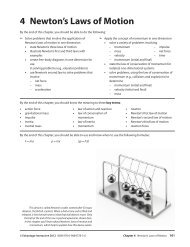
Figure 1.1.1 Galileo (top)<br />
<strong>and</strong> Newton<br />
Four hundred years ago, scientists were very interested in underst<strong>and</strong>ing <strong>the</strong> world<br />
around <strong>the</strong>m. There were hypo<strong>the</strong>ses about why <strong>the</strong> Sun came up each day or why<br />
objects fell to <strong>the</strong> ground, but <strong>the</strong>y were not based on evidence. Two physicists who used<br />
<strong>the</strong> scientific method to support <strong>the</strong>ir hypo<strong>the</strong>ses were <strong>the</strong> Italian Galileo Galilei (1564–<br />
1642) <strong>and</strong> <strong>the</strong> Englishman Sir Isaac Newton (1642–1727).<br />
Both Galileo <strong>and</strong> Newton provided insights into how our universe works on some<br />
fundamental principles. Galileo used evidence from his observations <strong>of</strong> planetary<br />
movement to support <strong>the</strong> idea that Earth revolved around <strong>the</strong> Sun. However, he was<br />
forced to deny this conclusion when put on trial. Eventually, his evidence was accepted<br />
as correct <strong>and</strong> we now consider Galileo one <strong>of</strong> <strong>the</strong> fa<strong>the</strong>rs <strong>of</strong> modern physics. Sir Isaac<br />
Newton, also considered one <strong>of</strong> <strong>the</strong> fa<strong>the</strong>rs <strong>of</strong> modern physics, was <strong>the</strong> first to describe<br />
motion <strong>and</strong> gravity. In this course, you will be introduced to his three laws <strong>of</strong> motion <strong>and</strong><br />
<strong>the</strong> universal law <strong>of</strong> gravitation. Both ideas form a foundation for classical physics. Like<br />
many o<strong>the</strong>rs that followed, both Galileo <strong>and</strong> Newton made <strong>the</strong>ir discoveries through<br />
careful observation, <strong>the</strong> collection <strong>of</strong> evidence, <strong>and</strong> interpretations based on that<br />
evidence.<br />
Different groups <strong>of</strong> scientists outline <strong>the</strong> parts <strong>of</strong> <strong>the</strong> scientific method in different<br />
ways. Here is one example, illustrating its steps.<br />
Steps <strong>of</strong> <strong>the</strong> Scientific Method<br />
1. Observation: Collection <strong>of</strong> data. Quantitative observation has numbers or<br />
quantities associated with it. Qualitative observation describes qualities or<br />
changes in <strong>the</strong> quality <strong>of</strong> matter including, for example, a substance’s colour,<br />
odour, or physical state.<br />
2. Statement <strong>of</strong> a hypo<strong>the</strong>sis: Formulation <strong>of</strong> a statement in an “if…<strong>the</strong>n…” format<br />
that explains <strong>the</strong> observations.<br />
3. Experimentation: Design <strong>and</strong> carry out a procedure to determine whe<strong>the</strong>r<br />
<strong>the</strong> hypo<strong>the</strong>sis accurately explains <strong>the</strong> observations. After making a set <strong>of</strong><br />
observations <strong>and</strong> formulating a hypo<strong>the</strong>sis, scientists devise an experiment.<br />
During <strong>the</strong> experiment <strong>the</strong>y carefully record additional observations. Depending<br />
on <strong>the</strong> results <strong>of</strong> <strong>the</strong> experiment, <strong>the</strong> hypo<strong>the</strong>sis may be adjusted <strong>and</strong><br />
experiments repeated to collect new observations many times.<br />
Sometimes <strong>the</strong> results <strong>of</strong> an experiment differ from what was expected.<br />
There are a variety <strong>of</strong> reasons this might happen. Things that contribute to such<br />
differences are called sources <strong>of</strong> error. They can include r<strong>and</strong>om errors over<br />
which <strong>the</strong> experimenter has no control <strong>and</strong> processes or equipment that can be<br />
adjusted, such as inaccurate measuring instruments. You will learn more about<br />
sources <strong>of</strong> error in experiments in section 1.3.<br />
4. Statement <strong>of</strong> a Theory: Statement <strong>of</strong> an explanation for <strong>the</strong> hypo<strong>the</strong>ses being<br />
investigated. Once enough information has been collected from a series <strong>of</strong><br />
experiments, a reasoned <strong>and</strong> coherent explanation called a <strong>the</strong>ory may be<br />
deduced. This <strong>the</strong>ory may lead to a model that helps us underst<strong>and</strong> <strong>the</strong> <strong>the</strong>ory.<br />
A model is usually a simplified description or representation <strong>of</strong> a <strong>the</strong>ory or<br />
phenomenon that can help us study it. Sometimes <strong>the</strong> scientific method leads<br />
to a law, which is a general statement <strong>of</strong> fact, without an accompanying set <strong>of</strong><br />
explanations.<br />
© Edvantage Interactive 2012 ISBN 978-0-9864778-3-6 Chapter 1 <strong>Skills</strong>, <strong>Methods</strong>, <strong>and</strong> <strong>the</strong> <strong>Nature</strong> <strong>of</strong> <strong>Physics</strong> 3
Quick Check<br />
1. What is <strong>the</strong> difference between a law <strong>and</strong> a <strong>the</strong>ory?<br />
______________________________________________________________________<br />
2. What are <strong>the</strong> fundamental steps <strong>of</strong> <strong>the</strong> scientific method?<br />
______________________________________________________________________<br />
______________________________________________________________________<br />
______________________________________________________________________<br />
______________________________________________________________________<br />
3. Classify <strong>the</strong> following observations as quantitative or qualitative by placing a checkmark in <strong>the</strong> correct<br />
column. Hint: Look at each syllable <strong>of</strong> those words: quantitative <strong>and</strong> qualitative. What do <strong>the</strong>y seem to<br />
mean?<br />
Observation<br />
Acceleration due to gravity is 9.8 m/s<br />
Quantitative Qualitative<br />
2 .<br />
A rocket travels faster than fighter jet.<br />
The density <strong>of</strong> sc<strong>and</strong>ium metal is 2.989 g/cm 3 .<br />
Copper metal can be used for wire to conduct electricity.<br />
Mass <strong>and</strong> velocity determine <strong>the</strong> momentum in an object.<br />
Zinc has a specific heat capacity <strong>of</strong> 388 J/(kg•K).<br />
The force applied to <strong>the</strong> soccer ball was 50 N.<br />
4. Use <strong>the</strong> steps <strong>of</strong> <strong>the</strong> scientific method to design a test for <strong>the</strong> following hypo<strong>the</strong>ses:<br />
(a) If cardboard is used to insulate a cup, it will keep a hot drink warmer.<br />
______________________________________________________________________<br />
______________________________________________________________________<br />
(b) If vegetable oil is used to grease a wheel, <strong>the</strong> wheel will turn faster.<br />
______________________________________________________________________<br />
______________________________________________________________________<br />
(c) If hot water is placed in ice cube trays, <strong>the</strong> water will freeze faster.<br />
______________________________________________________________________<br />
______________________________________________________________________<br />
4 Chapter 1 <strong>Skills</strong>, <strong>Methods</strong>, <strong>and</strong> <strong>the</strong> <strong>Nature</strong> <strong>of</strong> <strong>Physics</strong> © Edvantage Interactive 2012 ISBN 978-0-9864778-3-6
The Many Faces <strong>of</strong><br />
<strong>Physics</strong><br />
�����������������<br />
�� �� ��<br />
���������������<br />
�� ����<br />
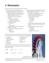
There are many different areas <strong>of</strong> study in <strong>the</strong> field <strong>of</strong> physics. Figure 1.1.2 gives an<br />
overview <strong>of</strong> <strong>the</strong> four main areas. Notice how <strong>the</strong> areas <strong>of</strong> study can be classified by two<br />
factors: size <strong>and</strong> speed. These two factors loosely describe <strong>the</strong> general <strong>the</strong>mes studied in<br />
each field. For example, this course focusses mainly classical mechanics, which involves<br />
relatively large objects <strong>and</strong> slow speeds.<br />
A quick Internet search will show you many different ways to classify <strong>the</strong> areas <strong>of</strong><br />
study within physics. The search will also show a new trend in <strong>the</strong> study <strong>of</strong> sciences, a<br />
trend that can have an impact on your future. Ra<strong>the</strong>r than working in one area <strong>of</strong> study or<br />
even within one discipline such as physics, biology, or chemistry, inter-disciplinary studies<br />
are becoming common. For example, an underst<strong>and</strong>ing <strong>of</strong> physics <strong>and</strong> biology might<br />
allow you to work in <strong>the</strong> area <strong>of</strong> biomechanics, which is <strong>the</strong> study <strong>of</strong> how <strong>the</strong> human<br />
muscles <strong>and</strong> bones work. Or maybe you will combine biology <strong>and</strong> physics to study<br />
exobiology, <strong>the</strong> study <strong>of</strong> life beyond <strong>the</strong> Earth’s atmosphere <strong>and</strong> on o<strong>the</strong>r planets.<br />
�������������<br />
������ �����<br />
Figure 1.1.2 The four main areas <strong>of</strong> physics. (Credit: Yassine Mrabet)<br />
�������������<br />
������ � ����<br />
© Edvantage Interactive 2012 ISBN 978-0-9864778-3-6 Chapter 1 <strong>Skills</strong>, <strong>Methods</strong>, <strong>and</strong> <strong>the</strong> <strong>Nature</strong> <strong>of</strong> <strong>Physics</strong> 5
1.2 Equipment Essentials<br />
Warm Up<br />
Your teacher will give you a pendulum made from some string <strong>and</strong> a washer. One swing <strong>of</strong> <strong>the</strong> pendulum back<br />
<strong>and</strong> forth is called a period <strong>and</strong> measured in seconds. Work with a partner to determine <strong>the</strong> period <strong>of</strong> your<br />
pendulum. Outline your procedure <strong>and</strong> results below. When you are done, identify one thing you would change<br />
in your procedure to improve your answer.<br />
Using a Calculator<br />
Quick Check<br />
A calculator is a tool that helps you perform calculations during investigations <strong>and</strong><br />
solving problems. You’ll have your calculator with you for every class. At <strong>the</strong> same time,<br />
however, you are not to rely on it exclusively. You need to underst<strong>and</strong> what <strong>the</strong> question<br />
is asking <strong>and</strong> what formula or calculation you need to use before you use your calculator.<br />
If you find yourself just pushing buttons to find an answer without underst<strong>and</strong>ing <strong>the</strong><br />
question, you need to talk to your teacher or a classmate to figure it out. Many times<br />
you’ll just need one concept clarified <strong>and</strong> <strong>the</strong>n you can solve <strong>the</strong> problem.<br />
Every calculator is different in terms <strong>of</strong> what order <strong>of</strong> buttons you need to push<br />
to find your answer. Use <strong>the</strong> Quick Check below to ensure you can find trigonometric<br />
functions <strong>and</strong> enter <strong>and</strong> manipulate exponents. If you cannot find <strong>the</strong> answers for <strong>the</strong>se<br />
questions, check with your teacher immediately.<br />
Using your calculator, what are <strong>the</strong> answers to <strong>the</strong> following ma<strong>the</strong>matical statements?<br />
1. sin 30° ________________________________ 4. (3.2 × 10 –4 ) × (2.5 × 10 6 )___________________________<br />
2. tan –1 .345 _____________________________ 5. pi – cos 60°_____________________________________<br />
3. 34 2 ___________________________________<br />
Measuring Time<br />
For objects that have a regularly repeated motion, each complete movement is called a<br />
cycle. The time during which <strong>the</strong> cycle is completed is called <strong>the</strong> period <strong>of</strong> <strong>the</strong> cycle. The<br />
number <strong>of</strong> cycles completed in one unit <strong>of</strong> time is called <strong>the</strong> frequency (ƒ) <strong>of</strong> <strong>the</strong> moving<br />
object. You may be familiar with <strong>the</strong> frequencies <strong>of</strong> several everyday objects. For example,<br />
a car engine may have a frequency <strong>of</strong> several thous<strong>and</strong> rpm (revolutions per minute).<br />
6 Chapter 1 <strong>Skills</strong>, <strong>Methods</strong>, <strong>and</strong> <strong>the</strong> <strong>Nature</strong> <strong>of</strong> <strong>Physics</strong> © Edvantage Interactive 2012 ISBN 978-0-9864778-3-6
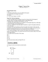
Figure 1.2.1 A recording timer that uses ticker tape to record<br />
time <strong>and</strong> distance<br />
Using a Motion<br />
Probe<br />
The turntable <strong>of</strong> an old phonograph record player may have frequencies <strong>of</strong> 33 rpm,<br />
45 rpm, or 78 rpm. A pendulum 24.85 cm long has a frequency <strong>of</strong> one cycle per second.<br />
Tuning forks may have frequencies such as 256 vibrations per second, 510 vibrations per<br />
second, <strong>and</strong> so on.<br />
Any measurement <strong>of</strong> time involves some sort <strong>of</strong> event that repeats itself at regular<br />
intervals. For example, a year is <strong>the</strong> time it takes Earth to revolve around <strong>the</strong> Sun; a day<br />
is <strong>the</strong> time it takes Earth to rotate on its axis; a month is approximately <strong>the</strong> time it takes<br />
<strong>the</strong> Moon to revolve around Earth. Perhaps moonth would be a better name for this time<br />
interval.<br />
All devices used to measure time contain some sort <strong>of</strong> regularly vibrating object<br />
such as a pendulum, a quartz crystal, a tuning fork, a metronome, or even vibrating<br />
electrons. With a pendulum you can experiment with <strong>the</strong> properties to make it a useful<br />
timing device. When a pendulum undergoes regularly repeated movements, each<br />
complete movement is called a cycle, <strong>and</strong> <strong>the</strong> time required for each cycle is called its<br />
period.<br />
A frequency <strong>of</strong> one cycle per second is called a hertz (Hz). Higher frequencies (such<br />
as radio signal frequencies) may be expressed in kilohertz (kHz) or even megahertz (MHz),<br />
where 1 kHz is 1000 Hz, <strong>and</strong> 1 MHz is 1 000 000 Hz.<br />
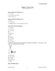
The Recording Timer<br />
In Investigation 1-1, you will use a device called a recording timer like <strong>the</strong> one in Figure<br />
1.2.1. The timer is a modified electric buzzer. A moving arm driven by an electromagnet<br />
vibrates with a constant frequency, <strong>and</strong> each time it<br />
vibrates, it strikes a piece <strong>of</strong> carbon paper. The carbon paper<br />
makes a small dot on a moving piece <strong>of</strong> ticker tape. The<br />
small dots are a record <strong>of</strong> both time <strong>and</strong> distance. If you<br />
know <strong>the</strong> frequency <strong>of</strong> vibration <strong>of</strong> <strong>the</strong> timer, you can figure<br />
out <strong>the</strong> period <strong>of</strong> time between <strong>the</strong> dots, because period (T)<br />
<strong>and</strong> frequency (ƒ) are reciprocals <strong>of</strong> one ano<strong>the</strong>r.<br />
T = 1/ƒ, <strong>and</strong> ƒ = 1/T<br />
If you measure <strong>the</strong> distance between <strong>the</strong> dots,<br />
this will tell you how far <strong>the</strong> object attached to <strong>the</strong> tape<br />
has moved. Knowing both distance <strong>and</strong> time, you can also<br />
calculate speed, since <strong>the</strong> speed <strong>of</strong> an object is <strong>the</strong> distance<br />
travelled divided by <strong>the</strong> time.<br />
Ano<strong>the</strong>r method for recording motion is a motion probe. There are several different<br />
models that can be used, but <strong>the</strong>y all follow <strong>the</strong> same basic principles. Using a computer<br />
or graphing calculator, <strong>the</strong> probe is plugged in <strong>and</strong> run via a s<strong>of</strong>tware program. The<br />
s<strong>of</strong>tware program collects data on <strong>the</strong> motion you are studying <strong>and</strong> represents <strong>the</strong>m as a<br />
graph on your computer screen.<br />
Using <strong>the</strong> data collected, you can analyze <strong>the</strong> motion. Your teacher will<br />
demonstrate how to use <strong>the</strong> motion probe in your lab.<br />
© Edvantage Interactive 2012 ISBN 978-0-9864778-3-6 Chapter 1 <strong>Skills</strong>, <strong>Methods</strong>, <strong>and</strong> <strong>the</strong> <strong>Nature</strong> <strong>of</strong> <strong>Physics</strong> 7
Investigation 1-1 Measuring <strong>the</strong> Frequency <strong>of</strong> a Recording Timer<br />
Purpose<br />
To measure <strong>the</strong> frequency <strong>of</strong> a recording timer <strong>and</strong> calculate its period<br />
Procedure<br />
1. Load <strong>the</strong> recording timer with a fresh piece <strong>of</strong> carbon paper. Pass a piece <strong>of</strong> ticker tape through <strong>the</strong> guiding<br />
staples, so that <strong>the</strong> carbon side <strong>of</strong> <strong>the</strong> paper faces <strong>the</strong> ticker tape. When <strong>the</strong> timer arm vibrates, it should leave a<br />
black mark on <strong>the</strong> tape.<br />
2. To measure <strong>the</strong> frequency <strong>of</strong> <strong>the</strong> recording timer, you must determine how many times <strong>the</strong> arm swings in<br />
1 s. Since it is difficult to time 1 s with any reasonable accuracy, let <strong>the</strong> timer run for 5 s, as precisely as you can<br />
measure it, <strong>the</strong>n count <strong>the</strong> number <strong>of</strong> carbon dots made on <strong>the</strong> tape <strong>and</strong> divide by 5. Practise moving <strong>the</strong> tape<br />
through <strong>the</strong> timer until you find a suitable speed that will spread <strong>the</strong> dots out for easy counting, but do not<br />
waste ticker tape.<br />
3. When you are ready, start <strong>the</strong> tape moving through <strong>the</strong> timer. Have your partner start <strong>the</strong> timer <strong>and</strong> <strong>the</strong><br />
stopwatch simultaneously. Stop <strong>the</strong> timer when 5 s have elapsed. Count <strong>the</strong> number <strong>of</strong> dots made in 5 s <strong>and</strong><br />
<strong>the</strong>n calculate <strong>the</strong> frequency <strong>of</strong> your timer in hertz (Hz).<br />
Concluding Questions<br />
1. What was <strong>the</strong> frequency <strong>of</strong> your recording timer in Hz?<br />
2. Estimate <strong>the</strong> possible error in <strong>the</strong> timing <strong>of</strong> your experiment. (It might be 0.10 s, 0.20 s, or whatever you think is<br />
likely.) Calculate <strong>the</strong> percent possible error in your timing. To do this, simply divide your estimate <strong>of</strong> <strong>the</strong> possible<br />
error in timing by 5.0 s <strong>and</strong> <strong>the</strong>n multiply by 100.<br />
Example: If you estimate your timing error to be 0.50 s, <strong>the</strong>n<br />
percent possible error in timing =<br />
8 Chapter 1 <strong>Skills</strong>, <strong>Methods</strong>, <strong>and</strong> <strong>the</strong> <strong>Nature</strong> <strong>of</strong> <strong>Physics</strong> © Edvantage Interactive 2012 ISBN 978-0-9864778-3-6<br />
0.50 s<br />
5.0 s<br />
× 100% = 10%<br />
3. Your calculated frequency will have <strong>the</strong> same percent possible error as you calculated for your timing error.<br />
Calculate <strong>the</strong> range within which your timer’s frequency probably falls.<br />
Example: If you calculate <strong>the</strong> frequency to be 57 Hz, <strong>and</strong> <strong>the</strong> possible error is 10%, <strong>the</strong>n <strong>the</strong> range is<br />
57 Hz + 5.7 Hz, or between 51.3 Hz <strong>and</strong> 62.7 Hz. Rounded <strong>of</strong>f, <strong>the</strong> range is between 51 Hz <strong>and</strong> 63 Hz.<br />
You might <strong>the</strong>refore conclude that <strong>the</strong> frequency <strong>of</strong> your timer is 57 + 6 Hz.<br />
4. If your timer operates on household voltage, its frequency (in North America) should be 60 Hz. Is 60 Hz within<br />
your estimated range for your timer?<br />
5. (a) What is <strong>the</strong> period <strong>of</strong> your timer?<br />
(b) How many dots on <strong>the</strong> ticker tape represent<br />
(i) 1.0 s?<br />
(ii) 0.10 s?
1.3 <strong>Physics</strong> Essentials<br />
Warm Up<br />
What is <strong>the</strong> difference between accuracy <strong>and</strong> precision? Explain your answer with real life examples.<br />
__________________________________________________________________________________<br />
__________________________________________________________________________________<br />
__________________________________________________________________________________<br />
Signi�cant Digits<br />
Imagine you are planning to paint a room in your house. To estimate how much paint<br />
you need to buy, you must know only <strong>the</strong> approximate dimensions <strong>of</strong> <strong>the</strong> walls. The<br />
rough estimate for one wall might be 8 m × 3 m. If, however, you are going to paste<br />
wallpaper on your wall <strong>and</strong> you require a neat, precise fit, you will probably make your<br />
measurements to <strong>the</strong> nearest millimetre. A proper measurement made for this purpose<br />
might look like this: 7.685 m × 2.856 m.<br />
Significant digits (“sig digs”) are <strong>the</strong> number <strong>of</strong> digits in <strong>the</strong> written value used to<br />
indicate <strong>the</strong> precision <strong>of</strong> a measurement. They are also called significant figures (“sig<br />
figs”). In <strong>the</strong> estimate <strong>of</strong> <strong>the</strong> wall size for determining how much paint is needed to<br />
cover a wall, <strong>the</strong> measurements (8 m × 3 m) have only one significant digit each. They<br />
are accurate to <strong>the</strong> nearest metre. In <strong>the</strong> measurements used to install wallpaper, <strong>the</strong><br />
measurements had four significant digits. They were accurate to <strong>the</strong> nearest millimetre.<br />
They were more precise.<br />
If you are planning to buy a very old used car, <strong>the</strong> salesman may ask you how much<br />
you want to spend. You might reply by giving him a rough estimate <strong>of</strong> around $600. This<br />
figure <strong>of</strong> $600 has one significant digit. You might write it as $600, but <strong>the</strong> zeros in this<br />
case are used simply to place <strong>the</strong> decimal point. When you buy <strong>the</strong> car <strong>and</strong> write a cheque<br />
for <strong>the</strong> full amount, you have to be more precise. For example, you might pay $589.96.<br />
This “measurement” has five significant digits. Of course, if you really did pay exactly $600,<br />
you would write <strong>the</strong> check for $600.00. In this case, all <strong>the</strong> zeros are measured digits, <strong>and</strong><br />
this measurement has five significant digits!<br />
You can see that zeros are sometimes significant digits (measured zeros) <strong>and</strong><br />
sometimes not. The measurer should make it clear whe<strong>the</strong>r <strong>the</strong> zeros are significant digits<br />
or just decimal-placing zeros. For example, you measure <strong>the</strong> length <strong>of</strong> a ticker tape to be<br />
7 cm, 3 mm, <strong>and</strong> around ½ mm long. How do you write down this measurement? You<br />
could write it several ways, <strong>and</strong> all are correct:<br />
7.35 cm, 73.5 mm, or 0.0735 m.<br />
Each <strong>of</strong> <strong>the</strong>se measurements is <strong>the</strong> same. Only <strong>the</strong> measuring units differ. Each<br />
measurement has three significant digits. The zeros in 0.0735 m are used only to place <strong>the</strong><br />
decimal.<br />
© Edvantage Interactive 2012 ISBN 978-0-9864778-3-6 Chapter 1 <strong>Skills</strong>, <strong>Methods</strong>, <strong>and</strong> <strong>the</strong> <strong>Nature</strong> <strong>of</strong> <strong>Physics</strong> 9
Accuracy <strong>and</strong><br />
Precision<br />
In ano<strong>the</strong>r example, <strong>the</strong> volume <strong>of</strong> a liquid is said to be 600 mL. How precise is this<br />
measurement? Did <strong>the</strong> measurer mean it was “around 600 mL”? Or was it 600 mL to <strong>the</strong><br />
nearest millilitre? Perhaps <strong>the</strong> volume was measured to <strong>the</strong> nearest tenth <strong>of</strong> a millilitre.<br />
Only <strong>the</strong> measurer really knows. Writing <strong>the</strong> volume as 600 mL is somewhat ambiguous.<br />
To be unambiguous, such a measurement might be expressed in scientific notation.<br />
To do this, <strong>the</strong> measurement is converted to <strong>the</strong> product <strong>of</strong> a number containing <strong>the</strong><br />
intended number <strong>of</strong> significant digits (using one digit to <strong>the</strong> left <strong>of</strong> <strong>the</strong> decimal point)<br />
<strong>and</strong> a power <strong>of</strong> 10. For example, if you write 6 × 10 2 mL, you are estimating to <strong>the</strong> nearest<br />
100 mL. If you write 6.0 × 10 2 mL, you are estimating to <strong>the</strong> nearest 10 mL.<br />
A measurement to <strong>the</strong> nearest millilitre would be 6.00 × 10 2 mL. The zeros here are<br />
measured zeros, not just decimal-placing zeros. They are significant digits.<br />
If it is not convenient to use scientific notation, you must indicate in some o<strong>the</strong>r<br />
way that a zero is a measured zero. For example, if <strong>the</strong> volume <strong>of</strong> a liquid is measured to<br />
<strong>the</strong> nearest mL to be “600.” mL, <strong>the</strong> decimal point will tell <strong>the</strong> reader that you measured<br />
to <strong>the</strong> nearest mL, <strong>and</strong> that both zeros are measured zeros. “600. mL” means <strong>the</strong> same as<br />
6.00 × 10 2 mL.<br />
The number <strong>of</strong> significant digits used to express <strong>the</strong> result <strong>of</strong> a measurement<br />
indicates how precise <strong>the</strong> measurement was. A person’s height measurement <strong>of</strong> 1.895 m<br />
is more precise than a measurement <strong>of</strong> 1.9 m.<br />
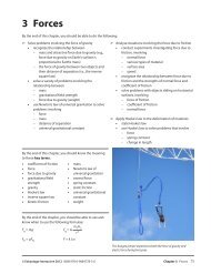
Measured values are determined using a variety <strong>of</strong> different measuring devices. There are<br />
devices designed to measure all sorts <strong>of</strong> different quantities. The collection pictured in<br />
Figure 1.3.1 measures temperature, length, <strong>and</strong> volume. In addition, <strong>the</strong>re are a variety <strong>of</strong><br />
precisions (exactnesses) associated with different devices. The micrometer (also called a<br />
caliper) is more precise than <strong>the</strong> ruler while <strong>the</strong> burette <strong>and</strong> pipette are more precise than<br />
<strong>the</strong> graduated cylinder.<br />
Figure 1.3.1 A selection <strong>of</strong> measuring devices with different<br />
levels <strong>of</strong> precision<br />
Despite <strong>the</strong> fact that some measuring devices are more precise than o<strong>the</strong>rs, it is<br />
impossible to design a measuring device that gives perfectly exact measurements. All<br />
measuring devices have some degree <strong>of</strong> uncertainty associated with <strong>the</strong>m.<br />
The 1-kg mass shown in Figure 1.3.2 is kept in a helium-filled bell jar at <strong>the</strong> BIPM<br />
in Sèvres France. It is <strong>the</strong> only exact mass on <strong>the</strong> planet. All o<strong>the</strong>r masses are measured<br />
relative to this <strong>and</strong> <strong>the</strong>refore have some degree <strong>of</strong> uncertainty associated with <strong>the</strong>m.<br />
10 Chapter 1 <strong>Skills</strong>, <strong>Methods</strong>, <strong>and</strong> <strong>the</strong> <strong>Nature</strong> <strong>of</strong> <strong>Physics</strong> © Edvantage Interactive 2012 ISBN 978-0-9864778-3-6
Figure 1.3.2 This kilogram mass was<br />
made in <strong>the</strong> 1880s. In 1889, it was<br />
accepted as <strong>the</strong> international prototype<br />
<strong>of</strong> <strong>the</strong> kilogram. (©BIPM — Reproduced<br />
with permission)<br />
Experimental Error<br />
Accuracy refers to <strong>the</strong> agreement <strong>of</strong> a particular value with<br />
<strong>the</strong> true value.<br />
Accurate measurements depend on careful design <strong>and</strong> calibration to<br />
ensure a measuring device is in proper working order. The term precision can<br />
actually have two different meanings.<br />
Precision refers to <strong>the</strong> reproducibility <strong>of</strong> a measurement or<br />
<strong>the</strong> agreement among several measurements <strong>of</strong> <strong>the</strong> same<br />
quantity.<br />
– or –<br />
Precision refers to <strong>the</strong> exactness <strong>of</strong> a measurement. This<br />
relates to uncertainty: <strong>the</strong> lower <strong>the</strong> uncertainty <strong>of</strong> a<br />
measurement, <strong>the</strong> higher <strong>the</strong> precision.<br />
A measurement can be very precise, yet very inaccurate. In 1895, a scientist<br />
estimated <strong>the</strong> time it takes planet Venus to rotate on its axis to be 23 h, 57 min, 36.2396 s.<br />
This is a very precise measurement! Unfortunately, it was found out later that <strong>the</strong> period<br />
<strong>of</strong> rotation <strong>of</strong> Venus is closer to 243 days! The latter measurement is much less precise, but<br />
probably a good deal more accurate!<br />
There is no such thing as a perfectly accurate measurement. Measurements are always<br />
subject to some uncertainty. Consider <strong>the</strong> following sources <strong>of</strong> experimental error.<br />
Systematic Errors<br />
Systematic errors may result from using an instrument that is in some way inaccurate.<br />
For example, if a wooden metre stick is worn at one end <strong>and</strong> you measure from this<br />
end, every reading will be too high. If an ammeter needle is not properly “zeroed,” all<br />
<strong>the</strong> readings taken with <strong>the</strong> meter will be too high or too low. Thermometers must be<br />
regularly checked for accuracy <strong>and</strong> corrections made to eliminate systematic errors in<br />
temperature readings.<br />
R<strong>and</strong>om Errors<br />
R<strong>and</strong>om errors occur in almost any measurement. For example, imagine you make five<br />
different readings <strong>of</strong> <strong>the</strong> length <strong>of</strong> a laboratory bench. You might obtain results such as:<br />
1.626 m, 1.628 m, 1.624 m, 1.626 m, <strong>and</strong> 1.625 m. You might average <strong>the</strong>se measurements<br />
<strong>and</strong> express <strong>the</strong> length <strong>of</strong> <strong>the</strong> bench in this way: 1.626 ± 0.002 m. This is a way <strong>of</strong> saying<br />
that your average measurement was 1.626 m, but <strong>the</strong> measurements, due to r<strong>and</strong>om<br />
errors, range between 1.624 m <strong>and</strong> 1.628 m.<br />
© Edvantage Interactive 2012 ISBN 978-0-9864778-3-6 Chapter 1 <strong>Skills</strong>, <strong>Methods</strong>, <strong>and</strong> <strong>the</strong> <strong>Nature</strong> <strong>of</strong> <strong>Physics</strong> <strong>11</strong>
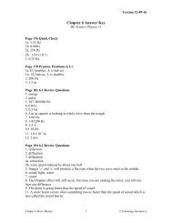
Quick Check<br />
Four groups <strong>of</strong> Earth <strong>Science</strong> students use <strong>the</strong>ir global positioning systems (GPS) to do some geocaching. The<br />
diagrams below show <strong>the</strong> students’ results relative to where <strong>the</strong> actual caches were located.<br />
������������<br />
��������<br />
����������<br />
1. Comment on <strong>the</strong> precision <strong>of</strong> <strong>the</strong> students in each <strong>of</strong> <strong>the</strong> groups. (In this case, we are using <strong>the</strong><br />
“reproducibility” definition <strong>of</strong> precision.)<br />
______________________________________________________________________________________<br />
2. What about <strong>the</strong> accuracy <strong>of</strong> each group?<br />
______________________________________________________________________________________<br />
3. Which groups were making systematic errors?<br />
______________________________________________________________________________________<br />
4. Which groups made errors that were more r<strong>and</strong>om?<br />
_______________________________________________________________________________________<br />
Figure 1.3.3 Observers A <strong>and</strong> B will make incorrect<br />
readings because <strong>of</strong> <strong>the</strong>ir positions relative to <strong>the</strong> ruler.<br />
�<br />
O<strong>the</strong>r Errors<br />
Regardless <strong>of</strong> <strong>the</strong> accuracy <strong>and</strong> precision <strong>of</strong> <strong>the</strong> measuring instrument, errors may arise<br />
when you, <strong>the</strong> experimenter, interact with <strong>the</strong> instrument. For example, if you measure<br />
<strong>the</strong> thickness <strong>of</strong> a piece <strong>of</strong> plastic using a micrometre caliper, your reading will be very<br />
precise but inaccurate if you tighten <strong>the</strong> caliper so much that you crush <strong>the</strong> plastic with<br />
<strong>the</strong> caliper!<br />
�<br />
A common personal error made by inexperienced<br />
�<br />
experimenters is failing to read scales with eye(s) in <strong>the</strong> proper<br />
position. In Figure 1.3.3, for example, only observer C will obtain <strong>the</strong><br />
correct measurement for <strong>the</strong> length <strong>of</strong> <strong>the</strong> block.<br />
12 Chapter 1 <strong>Skills</strong>, <strong>Methods</strong>, <strong>and</strong> <strong>the</strong> <strong>Nature</strong> <strong>of</strong> <strong>Physics</strong> © Edvantage Interactive 2012 ISBN 978-0-9864778-3-6
Combining<br />
Measurements<br />
Imagine that you have a laboratory bench that is 1.756 m long. The last digit (in italics)<br />
is an estimate to <strong>the</strong> nearest millimetre. You might call it an uncertain digit. Perhaps a<br />
truer measure might be 1.755 m or 1.757 m. Often you must estimate <strong>the</strong> last digit in a<br />
measurement when you guess what a reading is between <strong>the</strong> smallest divisions on <strong>the</strong><br />
measuring scale. This is true whe<strong>the</strong>r you are using a metre stick, a graduated cylinder, a<br />
chemical balance, or an ammeter.<br />
Adding or Subtracting Measurements<br />
Now imagine that you decide to add some thin plastic trim to <strong>the</strong> two ends <strong>of</strong> your<br />
bench. The trim has a width <strong>of</strong> 2.2 mm, which is 0.0022 m. What is <strong>the</strong> total length <strong>of</strong> <strong>the</strong><br />
bench with <strong>the</strong> new trim added?<br />
You add <strong>the</strong> widths <strong>of</strong> <strong>the</strong> two trimmed edges to <strong>the</strong> original length <strong>of</strong> <strong>the</strong> bench,<br />
like this:<br />
1.756 m<br />
0.0022 m<br />
0.0022 m<br />
1.7604 m = 1.760 m<br />
There is no point in carrying <strong>the</strong> last digit in <strong>the</strong> total. Since <strong>the</strong> 6 in 1.756 is<br />
uncertain, this makes <strong>the</strong> 0 in 1.7604 also uncertain, <strong>and</strong> <strong>the</strong> 4 following it a meaningless<br />
number. The proper way to write <strong>the</strong> total width <strong>of</strong> <strong>the</strong> bench is with just one uncertain<br />
digit, 1.760 m.<br />
Now imagine you have a graduated cylinder containing 12.00 mL <strong>of</strong> water.<br />
You carefully lower a glass marble into <strong>the</strong> graduated cylinder, <strong>and</strong> observe that <strong>the</strong> water<br />
level rises to 14.20 mL. What is <strong>the</strong> volume <strong>of</strong> <strong>the</strong> glass marble? To find out, you subtract<br />
<strong>the</strong> two measurements:<br />
14.20 mL<br />
–12.00 mL<br />
2.20 mL<br />
Notice that when <strong>the</strong> two measurements are subtracted, you lose a significant digit<br />
in this particular situation. What if <strong>the</strong> object added to <strong>the</strong> water was a small lead pellet<br />
<strong>and</strong> <strong>the</strong> volume increased from 12.00 mL to 12.20 mL? The volume <strong>of</strong> <strong>the</strong> pellet would<br />
be 0.20 mL. This measurement has only two significant digits. When measurements are<br />
subtracted, <strong>the</strong>re is <strong>of</strong>ten a loss <strong>of</strong> precision.<br />
Here is a common sense rule for adding or subtracting measurements:<br />
When adding or subtracting measurements, <strong>the</strong> sum or difference will have as many<br />
digits after <strong>the</strong> decimal point as <strong>the</strong> single measurement with <strong>the</strong> least number <strong>of</strong><br />
digits after <strong>the</strong> decimal point.<br />
© Edvantage Interactive 2012 ISBN 978-0-9864778-3-6 Chapter 1 <strong>Skills</strong>, <strong>Methods</strong>, <strong>and</strong> <strong>the</strong> <strong>Nature</strong> <strong>of</strong> <strong>Physics</strong> 13
Sample Problem 1.3.1 — Addition <strong>and</strong> Subtraction<br />
1. Add 4021.7 cm + 0.089 cm.<br />
2. Subtract 5643.92 m – 5643.7 m.<br />
What to Think About<br />
1. Addition<br />
1. Determine uncertain digits to be added.<br />
Indicated in bold italic type.<br />
2. Solve <strong>and</strong> report with <strong>the</strong> correct number <strong>of</strong><br />
digits after decimal <strong>the</strong> point.<br />
1. Subtraction<br />
1. Determine uncertain digits to be added.<br />
Indicated in bold.<br />
2. Solve <strong>and</strong> report with <strong>the</strong> correct number <strong>of</strong><br />
digits after <strong>the</strong> decimal point.<br />
3. Notice that <strong>the</strong> subtraction <strong>of</strong> two precise<br />
measurements has produced a very<br />
imprecise difference.<br />
How to Do It<br />
4021.7 cm<br />
+ 0.089 cm<br />
≅ 4021.8 cm<br />
5643.92 m<br />
– 5643.7 m<br />
≅ 0.2 m<br />
Practice Problems 1.3.1 — Addition <strong>and</strong> Subtraction<br />
Complete <strong>the</strong> following operations, using <strong>the</strong> rules for adding or subtracting measurements.<br />
1. 12.678 mm + 0.25 mm 4. 1.0001 mm – 0.1 mm<br />
2. 45.987 m 3 + 2.1 m 3 5. 12.5 g + 0.0005 g<br />
3. 12.345 mL – 0.34 mL 6. 16.768 kg – 1.0 g<br />
14 Chapter 1 <strong>Skills</strong>, <strong>Methods</strong>, <strong>and</strong> <strong>the</strong> <strong>Nature</strong> <strong>of</strong> <strong>Physics</strong> © Edvantage Interactive 2012 ISBN 978-0-9864778-3-6
Multiplying or Dividing Measurements<br />
You measure <strong>the</strong> dimensions <strong>of</strong> a wall to be 8.53 m × 2.74 m. What is <strong>the</strong> area <strong>of</strong> <strong>the</strong> wall?<br />
Imagine your calculator battery is dead, <strong>and</strong> you have to multiply <strong>the</strong> old-fashioned way.<br />
In <strong>the</strong> two measurements, <strong>the</strong> last digit is uncertain, so any product involving ei<strong>the</strong>r <strong>of</strong><br />
<strong>the</strong>se two digits will also be uncertain.<br />
8.53 m<br />
× 2.74 m<br />
3412<br />
5971<br />
1706<br />
23.3722 m 2 ≅ 23.4 m 2<br />
Since <strong>the</strong> 3 following <strong>the</strong> decimal is an uncertain digit, all digits following it are<br />
meaningless. Round <strong>of</strong>f <strong>the</strong> .3722 to .4, <strong>and</strong> write 23.4 m 2 for <strong>the</strong> area <strong>of</strong> <strong>the</strong> wall.<br />
Use <strong>the</strong> following common sense rule when multiplying or dividing measurements:<br />
When multiplying or dividing measurements, <strong>the</strong> product or quotient must have<br />
no more significant digits than <strong>the</strong> single measurement with <strong>the</strong> fewest significant<br />
digits. In o<strong>the</strong>r words, <strong>the</strong> least precise single measurement determines <strong>the</strong> precision<br />
<strong>of</strong> <strong>the</strong> final product or quotient.<br />
Sample Problem 1.3.2 — Multiplication <strong>and</strong> Division<br />
1. Multiply 2.54 cm × 5.08 cm.<br />
2. Divide 56.8 m 2 by 2.3 m.<br />
What to Think About<br />
1. Multiplication<br />
1. Determine uncertain digits. Indicated in bold.<br />
2. Multiple with calculator.<br />
3. Answer is not to correct number <strong>of</strong> significant digits.<br />
4. Solve <strong>and</strong> report with correct number <strong>of</strong> digits after<br />
decimal point. Remember to multiple units as well.<br />
2. Division<br />
1. Determine uncertain digits. Indicated in bold.<br />
2. Divide with calculator.<br />
3. Answer is not to correct number <strong>of</strong> significant digits.<br />
4. Solve <strong>and</strong> report with correct number <strong>of</strong> digits after<br />
decimal point. Remember to divide units as well.<br />
How to Do It<br />
2.54 cm × 5.08 cm<br />
12.9032 cm 2<br />
12.9 cm 2<br />
56.8 m 2 by 2.3 m<br />
24.695652<br />
25 m<br />
© Edvantage Interactive 2012 ISBN 978-0-9864778-3-6 Chapter 1 <strong>Skills</strong>, <strong>Methods</strong>, <strong>and</strong> <strong>the</strong> <strong>Nature</strong> <strong>of</strong> <strong>Physics</strong> 15
Practice Problems 1.3.2 — Multiplication <strong>and</strong> Division<br />
Perform <strong>the</strong> following operations, using <strong>the</strong> rule for multiplying <strong>and</strong> dividing measurements. Express answers in<br />
proper measuring units.<br />
1. 1.25 m × 0.25 m 4. 5.646 mL × 13.6 g/mL<br />
2. 3.987654 cm × 1.3 cm 5.<br />
3. 14.0 cm 2 ÷ 2.1 cm<br />
Scienti�c Notation<br />
Scientific notation is a convenient way to express numbers that are very large or very<br />
small. For example, one ampere <strong>of</strong> electric current is a measurement <strong>of</strong><br />
6 240 000 000 000 000 000 electrons passing a point in a wire in 1 s. This same number<br />
can be written, in scientific notation, as 6.24 × 10 18 electrons/second. This means 624<br />
followed by 16 zeros.<br />
Any number can be expressed in scientific notation. Here are some examples:<br />
0.10 = 1.0 × 10 -1<br />
1.0 = 1.0 × 10 0<br />
10.0 = 1.00 × 10 1<br />
100.0 = 1.000 × 10 2<br />
1 000.0 = 1.0000 × 10 3<br />
98.45 g/mL 5.762 mL<br />
1.4 mL<br />
16 Chapter 1 <strong>Skills</strong>, <strong>Methods</strong>, <strong>and</strong> <strong>the</strong> <strong>Nature</strong> <strong>of</strong> <strong>Physics</strong> © Edvantage Interactive 2012 ISBN 978-0-9864778-3-6
Quick Check<br />
1. Write <strong>the</strong> following measurements in scientific notation.<br />
(a) 0.00572 kg _____________________________ (d) 0.000 000 000 000 000 000 16 C ________________<br />
(b) 520 000 000 000 km _____________________ (e) <strong>11</strong>8.70004 g ________________________________<br />
(c) 300 000 000 m/s ________________________<br />
2. Simplify.<br />
(a) 10 3 × 10 7 × 10 12 _________________________<br />
(b) 10 23 ÷ 10 5 ______________________________<br />
(c) 10 12 × 10 –13 ____________________________<br />
(d) 10 –8 × 10 –12 ________________________________<br />
(e) 10 5 ÷ 10 –7 __________________________________<br />
(f) 10 –2 ÷ 10 –9 _________________________________<br />
3. Do <strong>the</strong> following calculations, <strong>and</strong> express your answers in scientific notation with <strong>the</strong> correct number <strong>of</strong><br />
significant digits.<br />
(a) (6.25 × 10 –7 ) ÷ (0.25 × 10 4 ) (c) 4.10 × 10 7 + 5.9 × 10 6<br />
(b) (93.8 × 10⁵ )(6.1 × 10 1 )<br />
(7.6 × 10 <strong>11</strong> )(1.22 × 10 7 )<br />
(d) (4.536 × 10 –3 ) – (0.347 × 10 –4 )<br />
4. A room has dimensions 13.48 m × 8.35 m × 3.18 m. What is its volume? Express your answer in scientific<br />
notation, with <strong>the</strong> correct number <strong>of</strong> significant digits.<br />
5. The volume <strong>of</strong> water in a graduated cylinder is 5.00 mL. A small lead sphere is gently lowered into <strong>the</strong><br />
graduated cylinder, <strong>and</strong> <strong>the</strong> volume rises to 5.10 mL. The mass <strong>of</strong> <strong>the</strong> lead sphere is 1.10 g. What is <strong>the</strong> density<br />
<strong>of</strong> <strong>the</strong> lead? (Density = mass/volume)<br />
© Edvantage Interactive 2012 ISBN 978-0-9864778-3-6 Chapter 1 <strong>Skills</strong>, <strong>Methods</strong>, <strong>and</strong> <strong>the</strong> <strong>Nature</strong> <strong>of</strong> <strong>Physics</strong> 17
Review <strong>of</strong> Basic Rules for H<strong>and</strong>ling Exponents<br />
Power <strong>of</strong> 10 Notation<br />
Multiplying Powers <strong>of</strong> 10<br />
Dividing Powers <strong>of</strong> 10<br />
0.000001 = 10 –6 1 = 10 0<br />
0.00001 = 10 –5 10 = 10 1<br />
0.0001 = 10 –4 100 = 10 2<br />
0.001 = 10 –3 1 000 = 10 3<br />
0.01 = 10 –2 10 000 = 10 4<br />
0.1 = 10 –1 100 000 = 10 5<br />
1 = 10 0 1 000 000 = 10 6<br />
Law <strong>of</strong> Exponents: a m . a n = a m+n<br />
(When multiplying, add exponents.)<br />
Examples: 100 × 1 000 = 10 2 • 10 3 = 10 5<br />
1<br />
100 × 1 000 = 10–2 × 10 3 = 10 1<br />
2500 × 4000 = 2.5 × 10 3 × 4.0 × 10 3 = 10 × 10 6 = 1.0 × 10 7<br />
Law <strong>of</strong> Exponents: am ÷ an = am – n<br />
(When dividing, subtract exponents.)<br />
Examples: 105<br />
10 = 105–1 = 10 4<br />
18 Chapter 1 <strong>Skills</strong>, <strong>Methods</strong>, <strong>and</strong> <strong>the</strong> <strong>Nature</strong> <strong>of</strong> <strong>Physics</strong> © Edvantage Interactive 2012 ISBN 978-0-9864778-3-6<br />
100<br />
1000<br />
1.00<br />
100 000<br />
102<br />
= = 10–1<br />
103 = 100<br />
= 10–5<br />
105
1.4 Analysis <strong>of</strong> Units <strong>and</strong> Conversions in <strong>Physics</strong><br />
Warm Up<br />
Place a check by <strong>the</strong> larger quantity in each row <strong>of</strong> <strong>the</strong> table.<br />
Metric Quantity Imperial Quantity<br />
A kilogram <strong>of</strong> butter A pound <strong>of</strong> butter<br />
A five-kilometre hiking<br />
trail<br />
A five-mile mountain bike<br />
trail<br />
One litre <strong>of</strong> milk One quart <strong>of</strong> milk<br />
A twelve-centimetre<br />
ruler<br />
A fifteen-gram piece <strong>of</strong><br />
chocolate<br />
A twelve-inch ruler<br />
A fifteen-ounce chocolate<br />
bar<br />
A temperature <strong>of</strong> 22°C A temperature <strong>of</strong> 22°F<br />
Measurement<br />
Through History<br />
Units <strong>of</strong> measurement were originally based on nature <strong>and</strong> everyday activities. The grain<br />
was derived from <strong>the</strong> mass <strong>of</strong> one grain <strong>of</strong> wheat or barley a farmer produced. The fathom<br />
was <strong>the</strong> distance between <strong>the</strong> tips <strong>of</strong> a sailor’s fingers when his arms were extended<br />
on ei<strong>the</strong>r side. The origin <strong>of</strong> units <strong>of</strong> length like <strong>the</strong> foot <strong>and</strong> <strong>the</strong> h<strong>and</strong> leave little to <strong>the</strong><br />
imagination.<br />
The inconvenient aspect <strong>of</strong> units such as <strong>the</strong>se was, <strong>of</strong> course, <strong>the</strong>ir glaring lack <strong>of</strong><br />
consistency. One “Viking’s embrace” might produce a fathom much shorter than ano<strong>the</strong>r.<br />
These inconsistencies were so important to traders <strong>and</strong> travellers that over <strong>the</strong> years most<br />
<strong>of</strong> <strong>the</strong> commonly used units were st<strong>and</strong>ardized. Eventually, <strong>the</strong>y were incorporated into<br />
what was known as <strong>the</strong> English units <strong>of</strong> measurement. Following <strong>the</strong> Battle <strong>of</strong> Hastings in<br />
1066, Roman measures were added to <strong>the</strong> primarily Anglo-Saxon ones that made up this<br />
system. These units were st<strong>and</strong>ardized by <strong>the</strong> Magna Carta <strong>of</strong> 1215 <strong>and</strong> were studied <strong>and</strong><br />
updated periodically until <strong>the</strong> UK Weights <strong>and</strong> Measures Act <strong>of</strong> 1824 resulted in a major<br />
review <strong>and</strong> a renaming to <strong>the</strong> Imperial system <strong>of</strong> measurement. It is interesting to<br />
note that <strong>the</strong> United States had become independent prior to this <strong>and</strong> did not adopt <strong>the</strong><br />
Imperial system, but continued to use <strong>the</strong> older English units <strong>of</strong> measure.<br />
Despite <strong>the</strong> st<strong>and</strong>ardization, development <strong>of</strong> this system from ancient agriculture<br />
<strong>and</strong> trade has led to a vast set <strong>of</strong> units that are quite complicated. For example, <strong>the</strong>re<br />
are eight different definitions for <strong>the</strong> amount <strong>of</strong> matter in a ton. The need for a simpler<br />
system, a system based on decimals, or multiples <strong>of</strong> 10, was recognized as early 1585<br />
when Flemish ma<strong>the</strong>matician Simon Stevin (1548–1620) published a book called The<br />
Tenth. However, most authorities credit Frenchman Gabriel Mouton (1618–1694) as <strong>the</strong><br />
originator <strong>of</strong> <strong>the</strong> metric system nearly 100 years later. Ano<strong>the</strong>r 100 years would pass<br />
before <strong>the</strong> final development <strong>and</strong> adoption <strong>of</strong> <strong>the</strong> metric system in France in 1795.<br />
© Edvantage Interactive 2012 ISBN 978-0-9864778-3-6 Chapter 1 <strong>Skills</strong>, <strong>Methods</strong>, <strong>and</strong> <strong>the</strong> <strong>Nature</strong> <strong>of</strong> <strong>Physics</strong> 19
Dimensional<br />
Analysis<br />
���� � � �<br />
����<br />
�<br />
Figure 1.4.2 A ruler with both<br />
imperial <strong>and</strong> metric scales shows<br />
that 1 inch = 2.54 cm.<br />
The International Bureau <strong>of</strong> Weights <strong>and</strong> Measures (BIPM) was established in Sévres,<br />
France, in 1825. The BIPM has governed <strong>the</strong> metric system ever since. Since 1960, <strong>the</strong><br />
metric system has become <strong>the</strong> International System <strong>of</strong> Units, known as <strong>the</strong> SI system. SI is<br />
from <strong>the</strong> French Système International. The SI system’s use <strong>and</strong> acceptance has grown to<br />
<strong>the</strong> point that only three countries in <strong>the</strong> entire world have not adopted it: Burma, Liberia,<br />
<strong>and</strong> <strong>the</strong> United States (Figure 1.4.1).<br />
������<br />
����������������<br />
�����������������<br />
��������������������<br />
�����������������<br />
�������<br />
Figure 1.4.1 Map <strong>of</strong> <strong>the</strong> world showing countries that have adopted <strong>the</strong> SI/metric system<br />
Dimensional analysis is a method that allows you to easily solve problems by converting<br />
from one unit to ano<strong>the</strong>r through <strong>the</strong> use <strong>of</strong> conversion factors. The dimensional analysis<br />
method is sometimes called <strong>the</strong> factor label method. It may occasionally be referred to as<br />
<strong>the</strong> use <strong>of</strong> unitary rates.<br />
A conversion factor is a fraction or factor written so that <strong>the</strong> denominator <strong>and</strong><br />
numerator are equivalent values with different units.<br />
One <strong>of</strong> <strong>the</strong> most useful conversion factors allows <strong>the</strong> user to convert from <strong>the</strong><br />
metric to <strong>the</strong> imperial system <strong>and</strong> vice versa. Since 1 inch is exactly <strong>the</strong> same length as<br />
2.54 cm, <strong>the</strong> factor may be expressed as:<br />
1 inch<br />
2.54 cm<br />
20 Chapter 1 <strong>Skills</strong>, <strong>Methods</strong>, <strong>and</strong> <strong>the</strong> <strong>Nature</strong> <strong>of</strong> <strong>Physics</strong> © Edvantage Interactive 2012 ISBN 978-0-9864778-3-6<br />
or<br />
�����<br />
2.54 cm<br />
1 inch<br />
These two lengths are identical so multiplication <strong>of</strong> a given length by <strong>the</strong><br />
conversion factor will not change <strong>the</strong> length. It will simply express it in a different unit<br />
(Figure 1.4.2).<br />
Now if you wish to determine how many centimetres are in a yard, you have<br />
two things to consider. First, which <strong>of</strong> <strong>the</strong> two forms <strong>of</strong> <strong>the</strong> conversion factor will allow<br />
you to cancel <strong>the</strong> imperial unit, converting it to a metric unit? Second, what o<strong>the</strong>r<br />
conversion factors will you need to complete <strong>the</strong> task?
Converting Within<br />
<strong>the</strong> Metric System<br />
Table 1.4.1 SI Prefixes<br />
Prefix Symbol 10 n<br />
yotta Y 1024 zetta Z 1021 exa E 1018 peta P 1015 tera T 1012 giga G 109 mega M 106 kilo k 103 hecto h 102 deca da 101 deci d 10-1 centi c 10 –2<br />
milli m 10 –3<br />
micro µ 10 –6<br />
nano n 10 –9<br />
pico p 10 –12<br />
femto f 10 –15<br />
atto a 10 –18<br />
zepto z 10 –21<br />
yocto y 10 –24<br />
Assuming you know, or can access, <strong>the</strong>se equivalencies: 1 yard = 3 feet <strong>and</strong> 1 foot =<br />
12 inches, your approach would be as follows:<br />
1.00 yards ×<br />
3 feet<br />
1 yard<br />
× 12 inches<br />
1 foot<br />
© Edvantage Interactive 2012 ISBN 978-0-9864778-3-6 Chapter 1 <strong>Skills</strong>, <strong>Methods</strong>, <strong>and</strong> <strong>the</strong> <strong>Nature</strong> <strong>of</strong> <strong>Physics</strong> 21<br />
× 2.54 cm<br />
1 inch<br />
= 91.4 cm<br />
Notice that as with <strong>the</strong> multiplication <strong>of</strong> any fractions, it is possible to cancel<br />
anything that appears in both <strong>the</strong> numerator <strong>and</strong> <strong>the</strong> denominator. We’ve simply<br />
followed a numerator-to-denominator pattern to convert yards to feet to inches to cm.<br />
The number <strong>of</strong> feet in a yard <strong>and</strong> inches in a foot are defined values. They are<br />
not things we measured. Thus <strong>the</strong>y do not affect <strong>the</strong> number <strong>of</strong> significant digits in<br />
our answer. This will be <strong>the</strong> case for any conversion factor in which <strong>the</strong> numerator <strong>and</strong><br />
denominator are in <strong>the</strong> same system (both metric or both imperial). Interestingly enough,<br />
<strong>the</strong> BIPM has indicated that 2.54 cm will be exactly 1 inch. So it is <strong>the</strong> only multiplesystem<br />
conversion factor that will not influence <strong>the</strong> number <strong>of</strong> significant digits in <strong>the</strong><br />
answer to a calculation. As all three <strong>of</strong> <strong>the</strong> conversion factors we used are defined, only<br />
<strong>the</strong> original value <strong>of</strong> 1.00 yards influences <strong>the</strong> significant digits in our answer. Hence we<br />
round <strong>the</strong> answer to three sig digs.<br />
The metric system is based on powers <strong>of</strong> 10. The power <strong>of</strong> 10 is indicated by a simple<br />
prefix. Table 1.4.1 is a list <strong>of</strong> SI prefixes. Your teacher will indicate those that you need to<br />
commit to memory. You may wish to highlight <strong>the</strong>m.<br />
Metric conversions require ei<strong>the</strong>r one or two steps. You will recognize a onestep<br />
metric conversion by <strong>the</strong> presence <strong>of</strong> a base unit in <strong>the</strong> question. The common<br />
base units in <strong>the</strong> metric system are shown in Table 1.4.2.<br />
Table 1.4.2 Common Metric Base Units<br />
Measures Unit Name Symbol<br />
length metre m<br />
mass gram g<br />
volume litre L<br />
time second s<br />
One-step metric conversions involve a base unit (metres, litres, grams, or<br />
seconds) being converted to a prefixed unit or a prefixed unit being converted to a<br />
base unit.<br />
Two-step metric conversions require <strong>the</strong> use <strong>of</strong> two conversion factors. Two<br />
factors will be required any time <strong>the</strong>re are two prefixed units in <strong>the</strong> question. In a<br />
two-step metric conversion, you must always convert to <strong>the</strong> base unit first.
Sample Problems 1.4.1— One- <strong>and</strong> Two-Step Metric Conversions<br />
1. Convert 9.4 nm into m. 2. Convert 6.32 μm into km.<br />
What to Think About<br />
Question 1<br />
1. In any metric conversion, you must decide<br />
whe<strong>the</strong>r you need one step or two. There is a<br />
base unit in <strong>the</strong> question <strong>and</strong> only one prefix.<br />
This problem requires only one step. Set <strong>the</strong><br />
units up to convert nm into m.<br />
Let <strong>the</strong> units lead you through <strong>the</strong> problem.<br />
You are given 9.4 nm, so <strong>the</strong> conversion<br />
factor must have nm in <strong>the</strong> denominator so it<br />
will cancel.<br />
2. Now determine <strong>the</strong> value <strong>of</strong> nano <strong>and</strong> fill it in<br />
appropriately. 1 nm = 10 –9 m<br />
Give <strong>the</strong> answer with <strong>the</strong> appropriate<br />
number <strong>of</strong> significant digits <strong>and</strong> <strong>the</strong> correct<br />
unit.<br />
Because <strong>the</strong> conversion factor is a defined<br />
equality, only <strong>the</strong> given value affects <strong>the</strong><br />
number <strong>of</strong> sig figs in <strong>the</strong> answer.<br />
Question 2<br />
1. This problem presents with two prefixes so<br />
<strong>the</strong>re must be two steps.<br />
The first step in such a problem is always to<br />
convert to <strong>the</strong> base unit. Set up <strong>the</strong> units to<br />
convert from μm to m <strong>and</strong> <strong>the</strong>n to km.<br />
2. Insert <strong>the</strong> values for 1 μm <strong>and</strong> 1 km.<br />
1 μm = 10 –6 m<br />
1 km = 10 3 m<br />
3. Give <strong>the</strong> answer with <strong>the</strong> correct number <strong>of</strong><br />
significant digits <strong>and</strong> <strong>the</strong> correct unit.<br />
How to Do It<br />
9.4 nm ×<br />
m<br />
nm = m<br />
9.4 nm × 10–9 m<br />
1 nm = 9.4 × 10⁻⁹ m<br />
6.32 μm ×<br />
6.32 μm × 10–6 m<br />
1 μm<br />
m<br />
μm ×<br />
km m = km<br />
× 1 km<br />
10 3 m = 6.32 × 10⁻⁹ km<br />
22 Chapter 1 <strong>Skills</strong>, <strong>Methods</strong>, <strong>and</strong> <strong>the</strong> <strong>Nature</strong> <strong>of</strong> <strong>Physics</strong> © Edvantage Interactive 2012 ISBN 978-0-9864778-3-6
Practice Problems 1.4.1 — One- <strong>and</strong> Two-Step Metric Conversions<br />
1. Convert 16 s into ks.<br />
2. Convert 75 000 mL into L.<br />
3. Convert 457 ks into ms.<br />
4. Convert 5.6 × 10 –4 Mm into dm.<br />
Derived Unit<br />
Conversions<br />
A derived unit is composed <strong>of</strong> more than one unit.<br />
Units like those used to express rate (km/h) or density (g/mL) are good examples <strong>of</strong><br />
derived units.<br />
Derived unit conversions require cancellations in two directions (from numerator to<br />
denominator as usual AND from denominator to numerator).<br />
Sample Problem 1.4.2 — Derived Unit Conversions<br />
Convert 55.0 km/h into m/s.<br />
What to Think About<br />
1. The numerator requires conversion <strong>of</strong> a<br />
prefixed metric unit to a base metric unit.<br />
This portion involves one step only <strong>and</strong> is<br />
similar to sample problem one above.<br />
2. The denominator involves a time conversion<br />
from hours to minutes to seconds. The<br />
denominator conversion usually follows <strong>the</strong><br />
numerator.<br />
Always begin by putting all conversion<br />
factors in place using units only. Now that<br />
this has been done, insert <strong>the</strong> appropriate<br />
numerical values for each conversion factor.<br />
3. As always, state <strong>the</strong> answer with units <strong>and</strong><br />
round to <strong>the</strong> correct number <strong>of</strong> significant<br />
digits (in this case, three).<br />
How to Do It<br />
55.0 km<br />
h × m<br />
km ×<br />
= m s<br />
55.0 km<br />
h<br />
× 103 m<br />
1 km × 1 h<br />
60 min<br />
= 15.3 m s<br />
The answer is 15.3 m/s.<br />
h<br />
min ×<br />
× 1 min<br />
60 s<br />
© Edvantage Interactive 2012 ISBN 978-0-9864778-3-6 Chapter 1 <strong>Skills</strong>, <strong>Methods</strong>, <strong>and</strong> <strong>the</strong> <strong>Nature</strong> <strong>of</strong> <strong>Physics</strong> 23<br />
min s
Practice Problems 1.4.2 — Derived Unit Conversions<br />
1. Convert 2.67 g/mL into kg/L. Why has <strong>the</strong> numerical value remained unchanged?<br />
2. Convert <strong>the</strong> density <strong>of</strong> neon gas from 8.9994 × 10 –4 mg/mL into kg/L.<br />
3. Convert 35 mi/h (just over <strong>the</strong> speed limit in a U.S. city) into m/s. (Given: 5280 feet = 1 mile)<br />
Use <strong>of</strong> a Value with a Derived Unit as a Conversion Factor<br />
A quantity expressed with a derived unit may be used to convert a unit that measures<br />
one thing into a unit that measures something else completely. The most common<br />
examples are <strong>the</strong> use <strong>of</strong> rate to convert between distance <strong>and</strong> time <strong>and</strong> <strong>the</strong> use <strong>of</strong> density<br />
to convert between mass <strong>and</strong> volume. These are challenging! The keys to this type <strong>of</strong><br />
problem are determining which form <strong>of</strong> <strong>the</strong> conversion factor to use <strong>and</strong> where to start.<br />
Suppose we wish to use <strong>the</strong> speed <strong>of</strong> sound (330 m/s) to determine <strong>the</strong> time (in<br />
hours) required for an explosion to be heard 5.0 km away. It is always a good idea to<br />
begin any conversion problem by considering what we are trying to find. Begin with <strong>the</strong><br />
end in mind. This allows us to decide where to begin. Do we start with 5.0 km or 330 m/s?<br />
First, consider: are you attempting to convert a unit → unit, or a unit<br />
unit<br />
→ unit<br />
unit ?<br />
As <strong>the</strong> answer is unit → unit, begin with <strong>the</strong> single unit: km. The derived unit will<br />
serve as <strong>the</strong> conversion factor.<br />
Second, which <strong>of</strong> <strong>the</strong> two possible forms <strong>of</strong> <strong>the</strong> conversion factor will allow<br />
330 m 1 s<br />
conversion <strong>of</strong> a distance in km into a time in h? Do we require or ? As <strong>the</strong><br />
1 s 330 m<br />
distance unit must cancel, <strong>the</strong> second form is <strong>the</strong> one we require. Hence, <strong>the</strong> correct<br />
approach is<br />
5.0 km × 103 m<br />
1 km<br />
1 s<br />
× ×<br />
1 min<br />
330 m 60 s<br />
× 1 h<br />
60 min = 4.2 × 10⁻³ h<br />
24 Chapter 1 <strong>Skills</strong>, <strong>Methods</strong>, <strong>and</strong> <strong>the</strong> <strong>Nature</strong> <strong>of</strong> <strong>Physics</strong> © Edvantage Interactive 2012 ISBN 978-0-9864778-3-6
Sample Problem 1.4.3 — Use <strong>of</strong> Density as a Conversion Factor<br />
What is <strong>the</strong> volume in L <strong>of</strong> a 15.0 kg piece <strong>of</strong> zinc metal? (Density <strong>of</strong> Zn = 7.13 g/mL)<br />
What to Think About<br />
1. Decide what form <strong>of</strong> <strong>the</strong> conversion factor to<br />
use: g/mL or <strong>the</strong> reciprocal, mL/g.<br />
Always begin by arranging <strong>the</strong> factors using<br />
units only. As <strong>the</strong> answer will contain one<br />
unit, begin with one unit, in this case, kg.<br />
2. Insert <strong>the</strong> appropriate numerical values for<br />
each conversion factor.<br />
In order to cancel a mass <strong>and</strong> convert to a<br />
volume, use <strong>the</strong> reciprocal <strong>of</strong> <strong>the</strong> density:<br />
1 mL<br />
7.13 g<br />
3. Calculate <strong>the</strong> answer with correct unit <strong>and</strong><br />
number <strong>of</strong> significant digits.<br />
How to Do It<br />
15.0 kg ×<br />
15.0 kg × 103 g<br />
1 kg<br />
g<br />
×<br />
mL<br />
kg g ×<br />
× 1 mL<br />
7.13 g × 10–3 L<br />
1 mL<br />
Practice Problems 1.4.3 — Use <strong>of</strong> Rate <strong>and</strong> Density as Conversion Factors<br />
1. The density <strong>of</strong> mercury metal is 13.6 g/mL. What is <strong>the</strong> mass <strong>of</strong> 2.5 L?<br />
L<br />
= ______ L<br />
mL<br />
= 2.10 L<br />
2. The density <strong>of</strong> lead is <strong>11</strong>.2 g/cm 3 . The volumes 1 cm 3 <strong>and</strong> 1 mL are exactly equivalent. What is <strong>the</strong> volume in<br />
litres <strong>of</strong> a 16.5 kg piece <strong>of</strong> lead?<br />
3. The speed <strong>of</strong> light is 3.0 × 10 10 cm/s. Sunlight takes 8.29 min to travel from <strong>the</strong> photosphere (light-producing<br />
region) <strong>of</strong> <strong>the</strong> Sun to Earth. How many kilometres is Earth from <strong>the</strong> Sun?<br />
1 m 3 ×<br />
Conversions Involving Units with Exponents (Ano<strong>the</strong>r Kind <strong>of</strong> Derived Unit)<br />
If a unit is squared or cubed, it may be cancelled in one <strong>of</strong> two ways. It may be written<br />
more than once to convey that it is being multiplied by itself or it may be placed in<br />
brackets with <strong>the</strong> exponent applied to <strong>the</strong> number inside <strong>the</strong> brackets as well as to <strong>the</strong><br />
unit. Hence, <strong>the</strong> use <strong>of</strong> <strong>the</strong> equivalency 1 L = 1 dm 3 to convert 1 m 3 to L might appear in<br />
ei<strong>the</strong>r <strong>of</strong> <strong>the</strong>se formats:<br />
1 dm<br />
10 –1 m<br />
× 1 dm<br />
10 –1 m<br />
× 1 dm<br />
10 –1 m ×<br />
1 L<br />
1 dm3 = 1 m3 × (<br />
1 dm<br />
10 –1 m ) 3<br />
×<br />
1 L<br />
1 dm 3<br />
= 1000 L<br />
© Edvantage Interactive 2012 ISBN 978-0-9864778-3-6 Chapter 1 <strong>Skills</strong>, <strong>Methods</strong>, <strong>and</strong> <strong>the</strong> <strong>Nature</strong> <strong>of</strong> <strong>Physics</strong> 25
Sample Problem 1.4.4 — Use <strong>of</strong> Conversion Factors Containing Exponents<br />
Convert 0.35 m 3 (cubic metres) into mL. (1 mL = 1 cm 3 )<br />
What to Think About<br />
1. The unit cm must be cancelled<br />
three times. Do this by multiplying<br />
<strong>the</strong> conversion factor by itself three<br />
times or through <strong>the</strong> use <strong>of</strong> brackets.<br />
2. Once <strong>the</strong> units have been aligned<br />
correctly, insert <strong>the</strong> appropriate<br />
numerical values.<br />
3. Calculate <strong>the</strong> answer with <strong>the</strong> correct<br />
unit <strong>and</strong> number <strong>of</strong> significant digits.<br />
How to Do It<br />
0.35 m 3 × cm m × cm m × cm m × mL<br />
cm 3<br />
= _________ mL<br />
or 0.35 m3 × (<br />
= _________ mL<br />
0.35 m3 1 cm<br />
×<br />
10 –2 m<br />
cm<br />
m ) 3<br />
×<br />
= 3.5 × 10⁵ mL<br />
or 0.35 m3 × 1 cm ( 10<br />
× 1 cm<br />
10 –2 m<br />
–2 m )3<br />
26 Chapter 1 <strong>Skills</strong>, <strong>Methods</strong>, <strong>and</strong> <strong>the</strong> <strong>Nature</strong> <strong>of</strong> <strong>Physics</strong> © Edvantage Interactive 2012 ISBN 978-0-9864778-3-6<br />
× 1 mL<br />
mL<br />
cm 3<br />
× 1 cm<br />
10 –2 m<br />
× 1 mL<br />
1 cm 3<br />
1 cm 3 = 3.5 × 10⁵ mL<br />
Practice Problems 1.4.4 — Use <strong>of</strong> Conversion Factors Containing Exponents<br />
1. Convert 4.3 dm3 into cm3 .<br />
2. Atmospheric pressure is 14.7 lb/in 2 . Convert this to <strong>the</strong> metric unit, g/cm 2 . (Given 454 g = 1.00 lb)<br />
3. Convert a density <strong>of</strong> 8.2 kg/m 3 to lb/ft 3 using factors provided in this section.
Graphing<br />
���<br />
���<br />
���<br />
���<br />
���<br />
�������<br />
���<br />
�<br />
��������<br />
In Figure 1.4.3, a variable y is plotted against a variable x. Variable y is <strong>the</strong> dependent<br />
variable <strong>and</strong> variable x is <strong>the</strong> independent variable. In this particular situation, <strong>the</strong> graph<br />
is a straight line. (You might say that variable y is a linear function <strong>of</strong> <strong>the</strong> variable x.)<br />
Figure 1.4.3 In a straight line graph like this one, <strong>the</strong> variable y is a linear function <strong>of</strong><br />
<strong>the</strong> variable x<br />
The slope <strong>of</strong> <strong>the</strong> graph is given <strong>the</strong><br />
symbol m, where m = rise<br />
run .<br />
To find <strong>the</strong> value <strong>of</strong> <strong>the</strong> slope, <strong>the</strong> two points with coordinates (0,b) <strong>and</strong> (x, y) will be<br />
used. The value <strong>of</strong> y where <strong>the</strong> graph intercepts <strong>the</strong> y-axis is called <strong>the</strong> y-intercept, <strong>and</strong> it<br />
is given <strong>the</strong> symbol b.<br />
�<br />
�����<br />
��������������������������������<br />
��������������� ��������������<br />
�����������<br />
�<br />
� �� ���� ���� ���� ���� ���� ���� ���� ���� ���� ����<br />
Figure 1.4.4 The slope <strong>of</strong> a line can be calculated using just two<br />
points.<br />
�������������<br />
����� ����� �<br />
�<br />
Since m = rise<br />
run<br />
= (y – b)<br />
(x – 0) ,<br />
Therefore, mx = y – b, or<br />
y = mx + b<br />
This is a general equation for any straight line. The<br />
slope <strong>of</strong> <strong>the</strong> line is m <strong>and</strong> <strong>the</strong> y-intercept is b.<br />
To write an equation for any straight-line graph,<br />
you need only determine <strong>the</strong> value <strong>of</strong> <strong>the</strong> y-intercept by<br />
inspection <strong>and</strong> <strong>the</strong> slope by calculation. You can <strong>the</strong>n<br />
substitute <strong>the</strong>se values into <strong>the</strong> general equation.<br />
For <strong>the</strong> linear graph in Figure 1.4.4, <strong>the</strong> y-intercept,<br />
by inspection, is 1.4. (b = 1.4) The slope is calculated using<br />
<strong>the</strong> two points with coordinates (0, 1.4) <strong>and</strong> (10.0, 4.4).<br />
© Edvantage Interactive 2012 ISBN 978-0-9864778-3-6 Chapter 1 <strong>Skills</strong>, <strong>Methods</strong>, <strong>and</strong> <strong>the</strong> <strong>Nature</strong> <strong>of</strong> <strong>Physics</strong> 27<br />
m =<br />
(4.4 – 1.4)<br />
(10.0 – 0)<br />
3.0<br />
= = 0.30<br />
10.0<br />
The equation for this straight line is <strong>the</strong>refore: y = 0.30 x + 1.4<br />
In <strong>the</strong>se examples, <strong>the</strong> units <strong>of</strong> measure <strong>of</strong> <strong>the</strong> variables have not been included,<br />
in order to simplify <strong>the</strong> explanation. In experiments, <strong>the</strong> observations you make are<br />
frequently summarized in graphical form. When graphing experimental data, always<br />
include <strong>the</strong> measuring units <strong>and</strong> <strong>the</strong> specific symbols <strong>of</strong> <strong>the</strong> variables being graphed.<br />
������
�������<br />
���<br />
���<br />
���<br />
���<br />
���<br />
�<br />
� �� ���� ���� ���� ���� ����<br />
����������<br />
��������������<br />
���������������������<br />
������������������<br />
Figure 1.4.5 Three common types <strong>of</strong> graphic relationships<br />
The three most common types <strong>of</strong> graphic relationships are shown in Figure 1.4.5.<br />
���������������<br />
���<br />
���<br />
���<br />
���<br />
���<br />
�<br />
� �� ���� ���� ���� ���� ���� ���<br />
�������������<br />
����������������<br />
�����������������������������<br />
Sample Problem 1.4.5 — Determination <strong>of</strong> a Relationship from Data<br />
Find <strong>the</strong> relationship for <strong>the</strong> graphed data below:<br />
����������������<br />
��<br />
��<br />
��<br />
�����������������<br />
��<br />
�<br />
�<br />
������<br />
�<br />
� � �� �� �� �� ��� ��� ��� ��� ��� ��<br />
�������������<br />
�<br />
������<br />
What to Think About<br />
1. Determine <strong>the</strong> slope for <strong>the</strong> straight line. To do<br />
this, select two points on <strong>the</strong> line <strong>of</strong> best fit.<br />
These should be points whose values are easy<br />
to determine on both axes. Do not use data<br />
points to determine <strong>the</strong> constant.<br />
Determine <strong>the</strong> change in y (Δy) <strong>and</strong> <strong>the</strong> change<br />
in x (∆x) including <strong>the</strong> units.<br />
The constant is ∆y/ ∆x.<br />
2. Determine <strong>the</strong> relationship by subbing <strong>the</strong><br />
variable names <strong>and</strong> <strong>the</strong> constant into <strong>the</strong><br />
general equation, y = mx + b.<br />
Often, a straight line graph passes through <strong>the</strong><br />
origin, in which case, y = mx.<br />
How to Do It<br />
∆y is 25–5 = 20 m<br />
∆x is 18 – 1 = 17 s<br />
20 m<br />
17 s<br />
= 1.18 m/s<br />
28 Chapter 1 <strong>Skills</strong>, <strong>Methods</strong>, <strong>and</strong> <strong>the</strong> <strong>Nature</strong> <strong>of</strong> <strong>Physics</strong> © Edvantage Interactive 2012 ISBN 978-0-9864778-3-6<br />
�<br />
�����������<br />
�<br />
�<br />
�<br />
� �� �� �� �� �� �<br />
������������<br />
������������������� �<br />
�����������������������������<br />
�������������<br />
distance = (1.18 m/s)time + 4.0 m/s.
Practice Problems 1.4.5 — Determination <strong>of</strong> a Relationship from Data<br />
1. Examine <strong>the</strong> following graphs. What type <strong>of</strong> relationship does each represent? Give <strong>the</strong> full relationship<br />
described by graph (c).<br />
�����������<br />
���������������<br />
����������������<br />
��<br />
��<br />
��<br />
��<br />
��<br />
��<br />
��<br />
��<br />
��<br />
����������<br />
�������������<br />
�<br />
� �� �� �� �� �� �� �� �� �� �� ��<br />
�������������<br />
2. A beaker full <strong>of</strong> water is placed on a hotplate <strong>and</strong> heated over a period <strong>of</strong> time. The temperature is recorded<br />
at regular intervals. The following data was collected. Use <strong>the</strong> following grid to plot a graph <strong>of</strong> temperature<br />
against time. (Time goes on <strong>the</strong> x-axis.)<br />
Temperature ( o C) Time (min)<br />
22 0<br />
30 2<br />
38 4<br />
46 6<br />
54 8<br />
62 10<br />
70 12<br />
Continued on <strong>the</strong> next page<br />
© Edvantage Interactive 2012 ISBN 978-0-9864778-3-6 Chapter 1 <strong>Skills</strong>, <strong>Methods</strong>, <strong>and</strong> <strong>the</strong> <strong>Nature</strong> <strong>of</strong> <strong>Physics</strong> 29
Practice Problems 1.4.5 — Determination <strong>of</strong> a Relationship from Data (Continued)<br />
(a) What type <strong>of</strong> relationship was studied during this investigation?<br />
(b) What is <strong>the</strong> constant (be sure to include <strong>the</strong> units)?<br />
(c) What temperature was reached at 5 min?<br />
(d) Use <strong>the</strong> graph to determine <strong>the</strong> relationship between temperature <strong>and</strong> time.<br />
(e) How long would it take <strong>the</strong> temperature to reach 80°C?<br />
(f) What does <strong>the</strong> y-intercept represent?<br />
(g) Give a source <strong>of</strong> error that might cause your graph to vary from that expected.<br />
30 Chapter 1 <strong>Skills</strong>, <strong>Methods</strong>, <strong>and</strong> <strong>the</strong> <strong>Nature</strong> <strong>of</strong> <strong>Physics</strong> © Edvantage Interactive 2012 ISBN 978-0-9864778-3-6
Investigation 1-4 Making a Pendulum Clock<br />
Purpose<br />
To learn how a pendulum can be used as a clock<br />
Procedure<br />
1. Prepare a simple pendulum by tying a string to a pendulum bob, ei<strong>the</strong>r a large washer, as in Figure 1.4.6, or<br />
a drilled metal ball. Feed <strong>the</strong> string through <strong>the</strong> opening <strong>of</strong> <strong>the</strong> pendulum support. Avoid winding <strong>the</strong> string<br />
around <strong>the</strong> support rod. If you do this, <strong>the</strong> length <strong>of</strong> <strong>the</strong> pendulum changes during a swing.<br />
����<br />
�������<br />
�����������<br />
����������<br />
Figure 1.4.6 Setup for Investigation 1-4<br />
����������<br />
�<br />
2. Start by adjusting <strong>the</strong> length l <strong>of</strong> <strong>the</strong> pendulum so that it is as close to being 10.00 cm as you can make it.<br />
Measure l from <strong>the</strong> bottom <strong>of</strong> <strong>the</strong> pendulum clamp to <strong>the</strong> centre <strong>of</strong> <strong>the</strong> bob, as shown in Figure 1.4.6.<br />
3. Push <strong>the</strong> bob a small distance, about 2 cm, to one side <strong>and</strong> let it swing freely. To get a rough idea <strong>of</strong> how long<br />
<strong>the</strong> pendulum takes to make one swing, use a stopwatch to measure <strong>the</strong> time it takes for <strong>the</strong> bob to swing<br />
from <strong>the</strong> highest point on one side <strong>of</strong> <strong>the</strong> swing to <strong>the</strong> highest point on <strong>the</strong> o<strong>the</strong>r side, <strong>the</strong>n back to its starting<br />
position. The time it takes <strong>the</strong> pendulum bob to complete a full swing like this is called <strong>the</strong> period (T) <strong>of</strong> <strong>the</strong><br />
pendulum. Try measuring <strong>the</strong> period <strong>of</strong> one swing several times with your stopwatch. Why do you think your<br />
measurements are so inconsistent?<br />
4. To obtain a more reliable measurement <strong>of</strong> <strong>the</strong> period <strong>of</strong> <strong>the</strong> pendulum, you will now measure <strong>the</strong> time for<br />
a large number <strong>of</strong> swings (50) <strong>and</strong> find <strong>the</strong> average time for one swing by dividing by 50. Set your 10.00 cm<br />
pendulum swinging through a small arc, as before. Start counting backward (3, 2, 1, 0, 1, 2, 3, 4, etc.) <strong>and</strong> start<br />
your stopwatch at 0. Stop your watch after 50 swings <strong>and</strong> record <strong>the</strong> time your pendulum took to complete<br />
50 swings.<br />
5. To figure out <strong>the</strong> period <strong>of</strong> <strong>the</strong> pendulum, divide <strong>the</strong> time for 50 swings by 50.0. Record <strong>the</strong> period, T, in a table<br />
like Table 1.4.3. Check your result by repeating <strong>the</strong> measurement. If necessary, repeat a third time.<br />
© Edvantage Interactive 2012 ISBN 978-0-9864778-3-6 Chapter 1 <strong>Skills</strong>, <strong>Methods</strong>, <strong>and</strong> <strong>the</strong> <strong>Nature</strong> <strong>of</strong> <strong>Physics</strong> 31
6. Measure <strong>the</strong> period <strong>of</strong> your pendulum for each <strong>of</strong> <strong>the</strong> lengths in Table 1.4.3. Record all your results in Table 1.4.3.<br />
7. Prepare a graph with headings <strong>and</strong> labels like those in Figure 1.4.7. In this experiment, <strong>the</strong> period <strong>of</strong> <strong>the</strong><br />
pendulum depends on its length, so <strong>the</strong> period is called <strong>the</strong> dependent variable. The dependent variable goes<br />
on <strong>the</strong> y-axis. Length is <strong>the</strong> independent variable. We chose what its values would be. Length is on <strong>the</strong> x-axis.<br />
Plot period against length using all your data from Table 1.4.3. Use a small dot with a circle around it to make<br />
each position more visible. See Figure 1.4.7 for a sample point. When you have plotted all <strong>the</strong> points, draw one<br />
smooth curve through as many <strong>of</strong> <strong>the</strong> points as possible. If one or two points are obvious errors, ignore <strong>the</strong>m<br />
when drawing your curve.<br />
8. Make pendulums with <strong>the</strong> lengths you obtain from your graph for pendulums with periods <strong>of</strong> 1.0 s <strong>and</strong> 2.0 s.<br />
See if <strong>the</strong> lengths predicted by <strong>the</strong> graph actually do produce 1.0 s <strong>and</strong> 2.0 s “clocks.”<br />
Table 1.4.3 Data Table<br />
Length <strong>of</strong><br />
Pendulum,<br />
l (cm)<br />
10.00<br />
15.00<br />
20.00<br />
25.00<br />
30.00<br />
40.00<br />
50.00<br />
60.00<br />
70.00<br />
80.00<br />
90.00<br />
100.0<br />
Time for<br />
50 Swings<br />
(s)<br />
Time for<br />
1 Swing,<br />
Period, T<br />
(s)<br />
�<br />
� �� ����� ����� ����� ����� ����� ����� ����� ����� ����� �����<br />
Concluding Questions<br />
1. According to your graph <strong>of</strong> period vs. length, how long must your pendulum be if it is to be used as (a) a “onesecond<br />
clock”? (b) a “two-second clock”? (Such a pendulum takes 1s to swing one way, <strong>and</strong> one second to swing<br />
back.)<br />
2. To increase <strong>the</strong> period <strong>of</strong> your pendulum from 1 s to 2 s, by how many times (to <strong>the</strong> nearest whole number)<br />
must you increase its length?<br />
Challenges<br />
1. Predict what length a 3.0 s pendulum clock would have to be. Test your prediction by experiment.<br />
2. Predict what will happen to <strong>the</strong> period <strong>of</strong> a pendulum if you double <strong>the</strong> mass <strong>of</strong> <strong>the</strong> pendulum bob. Test your<br />
prediction.<br />
3. Will <strong>the</strong> period <strong>of</strong> a pendulum change after it has been swinging for a while? Test your answer by<br />
experimenting!<br />
32 Chapter 1 <strong>Skills</strong>, <strong>Methods</strong>, <strong>and</strong> <strong>the</strong> <strong>Nature</strong> <strong>of</strong> <strong>Physics</strong> © Edvantage Interactive 2012 ISBN 978-0-9864778-3-6<br />
�������������<br />
����<br />
����<br />
����<br />
����<br />
����<br />
����<br />
�������������������������������<br />
��������������<br />
Figure 1.4.7 Label your graph as shown here.<br />
������������
1.5 Vectors<br />
Warm Up<br />
Your teacher will place an object in <strong>the</strong> classroom. Use only written directions to explain to someone who is<br />
blindfolded how to get from your chair to <strong>the</strong> object.<br />
_________________________________________________________________________________________<br />
_________________________________________________________________________________________<br />
_________________________________________________________________________________________<br />
Introduction to<br />
Vectors<br />
Figure 1.5.2 The cardinal<br />
directions are north, east,<br />
south, <strong>and</strong> west, as shown on<br />
this compass.<br />
���<br />
���<br />
���<br />
������<br />
�����<br />
��� ���<br />
����<br />
Figure 1.5.1 Buddy’s trip around <strong>the</strong> front yard<br />
© Edvantage Interactive 2012 ISBN 978-0-9864778-3-6 Chapter 1 <strong>Skills</strong>, <strong>Methods</strong>, <strong>and</strong> <strong>the</strong> <strong>Nature</strong> <strong>of</strong> <strong>Physics</strong> 33<br />
���<br />
���<br />
In Figure 1.5.1, notice a series <strong>of</strong> arrows drawn on <strong>the</strong> map <strong>of</strong> a physics teacher’s<br />
front lawn. Each arrow shows <strong>the</strong> magnitude (size) <strong>and</strong> direction <strong>of</strong> a series <strong>of</strong> successive<br />
trips made by Buddy, <strong>the</strong> teacher’s dog. Buddy was “doing his thing” before getting into<br />
<strong>the</strong> car for a trip to school. These arrows, showing both magnitude <strong>and</strong> direction <strong>of</strong> each<br />
<strong>of</strong> Buddy’s displacements, are called vectors.<br />
To identify <strong>the</strong> direction <strong>of</strong> vectors, two common conventions are used: numerical<br />
<strong>and</strong> compass. Sometimes compass directions are also called cardinal directions.<br />
Numerical directions use a positive <strong>and</strong> negative sign to indicate direction. If you<br />
think <strong>of</strong> a graph, <strong>the</strong> “up” direction on <strong>the</strong> y-axis <strong>and</strong> <strong>the</strong> “right” direction on <strong>the</strong> x-axis are<br />
positive. “Down” on <strong>the</strong> y-axis <strong>and</strong> “left” on <strong>the</strong> x-axis is negative. For example, a person<br />
walking 2 km right is walking +2 km <strong>and</strong> a person walking 2 km left is walking –2 km. The<br />
sign indicates direction.<br />
Compass or cardinal directions are ano<strong>the</strong>r way <strong>of</strong> indicating vector directions. As<br />
Figure 1.5.2 shows, <strong>the</strong>re are four main directions on <strong>the</strong> compass: north, east, south, <strong>and</strong><br />
west. North <strong>and</strong> west are usually positive, <strong>and</strong> east <strong>and</strong> south are negative. For example, if<br />
a person walking north encounters a person walking south, <strong>the</strong> two people are walking in<br />
opposite directions.
To determine <strong>the</strong> angle θ, you use trigonometric ratios. Three trigonometric<br />
ratios are particularly useful for solving vector problems. In <strong>the</strong> right-angled triangle<br />
A<strong>BC</strong>, consider <strong>the</strong> angle labelled θ. With reference to θ, AC is <strong>the</strong> opposite side (o), <strong>BC</strong><br />
is <strong>the</strong> adjacent side (a), <strong>and</strong> AB is <strong>the</strong> hypotenuse (h). In any right-angled triangle, <strong>the</strong><br />
hypotenuse is always <strong>the</strong> side opposite to <strong>the</strong> right angle.<br />
�<br />
��������������<br />
�<br />
�����������������<br />
�����������������<br />
Figure 1.5.3 The sides <strong>of</strong> a right-angled triangle are used to<br />
define trigonometric ratios.<br />
34 Chapter 1 <strong>Skills</strong>, <strong>Methods</strong>, <strong>and</strong> <strong>the</strong> <strong>Nature</strong> <strong>of</strong> <strong>Physics</strong> © Edvantage Interactive 2012 ISBN 978-0-9864778-3-6<br />
�<br />
�<br />
The three most commonly used trigonometric ratios are defined as follows:<br />
sine θ =<br />
cosine θ =<br />
tangent θ =<br />
opposite side<br />
hypotenuse<br />
adjacent side<br />
hypotenuse<br />
= o<br />
h<br />
opposite side<br />
adjacent side<br />
= a<br />
h<br />
= o<br />
a<br />
Trigonometric ratios can help you solve vector problems quickly <strong>and</strong> accurately.<br />
Scientific calculators can provide you with <strong>the</strong> ratios for any angle.<br />
Now, back to Figure 1.5.1. When Buddy reaches his final spot near <strong>the</strong> car door, how<br />
far has he walked since he left <strong>the</strong> front porch? This question has two answers, depending<br />
on what “How far?” means. The distance Buddy has travelled is <strong>the</strong> arithmetic sum <strong>of</strong> all<br />
<strong>the</strong> short distances he has travelled between <strong>the</strong> shrubs, trees, <strong>and</strong> fire hydrant while he<br />
visited <strong>the</strong>m. This is simple to calculate.<br />
total distance = 3.0 m + 2.0 m + 4.0 m + 4.0 m + 2.0 m + 4.0 m = 19.0 m<br />
If, however, you want to know how far Buddy has travelled from <strong>the</strong> porch, <strong>the</strong><br />
bold line in Figure 1.1.5, <strong>the</strong>n you want to know Buddy’s displacement. It turns out<br />
that Buddy’s displacement from <strong>the</strong> front porch is 5.0 m. The bold arrow represents <strong>the</strong><br />
magnitude (5.0 m) <strong>and</strong> <strong>the</strong> direction (53° to <strong>the</strong> right <strong>of</strong> his starting direction) <strong>of</strong> Buddy’s<br />
displacement, <strong>and</strong> is called <strong>the</strong> resultant displacement. The resultant displacement is<br />
not <strong>the</strong> arithmetic sum, but <strong>the</strong> vector sum <strong>of</strong> <strong>the</strong> individual displacement vectors shown<br />
on <strong>the</strong> diagram.<br />
There are two ways to indicate that a quantity is a vector quantity. The best way<br />
is to include a small arrow above <strong>the</strong> symbol for <strong>the</strong> vector quantity. For example,<br />
Δd → symbolizes a displacement vector. If it’s not possible to include <strong>the</strong> arrow when<br />
typing, a vector quantity may be typed in bold italics. For example, Δd also symbolizes a<br />
displacement vector. If only <strong>the</strong> magnitude <strong>of</strong> <strong>the</strong> vector is <strong>of</strong> importance, <strong>the</strong> symbol Δd<br />
(no arrow or not bold) is used.
Adding Vectors<br />
Scalars <strong>and</strong> Vectors<br />
Free Body Diagrams<br />
Draw <strong>the</strong> first vector to scale <strong>and</strong> in <strong>the</strong> proper direction. Draw <strong>the</strong> second vector to scale,<br />
beginning at <strong>the</strong> tip <strong>of</strong> <strong>the</strong> first vector, <strong>and</strong> in <strong>the</strong> proper direction. Add <strong>the</strong> third vector (if<br />
<strong>the</strong>re is one), beginning at <strong>the</strong> tip <strong>of</strong> <strong>the</strong> second vector. Repeat this procedure until all <strong>the</strong><br />
vectors have been added. The vector sum or resultant <strong>of</strong> all <strong>the</strong> vectors is <strong>the</strong> vector that<br />
starts at <strong>the</strong> tail <strong>of</strong> <strong>the</strong> first vector <strong>and</strong> ends at <strong>the</strong> tip <strong>of</strong> <strong>the</strong> last vector.<br />
This is what was done in Figure 1.5.1. The resultant displacement <strong>of</strong> Buddy is<br />
correctly written as 5.0 m, 53° to <strong>the</strong> right <strong>of</strong> his starting direction.<br />
If you add 3 kg <strong>of</strong> sugar to 2 kg <strong>of</strong> sugar, you will have 5 kg <strong>of</strong> sugar. If you add 3 L <strong>of</strong> water<br />
to 2 L <strong>of</strong> water, you will have 5 L <strong>of</strong> water. Masses <strong>and</strong> volumes are added toge<strong>the</strong>r by <strong>the</strong><br />
rules <strong>of</strong> ordinary arithmetic. Mass <strong>and</strong> volume are scalar quantities. Scalar quantities<br />
have magnitude but no direction. O<strong>the</strong>r scalar quantities include: distance, speed, time,<br />
energy, <strong>and</strong> density.<br />
If you add a 3 m displacement to a 2 m displacement, <strong>the</strong> two displacements<br />
toge<strong>the</strong>r may add up to 5 m, but <strong>the</strong>y may also add up to 1 m or any magnitude between<br />
1 m <strong>and</strong> 5 m! Figure 1.5.2 shows some <strong>of</strong> <strong>the</strong> ways <strong>the</strong>se displacements might add up. In<br />
Figure 1.5.4, <strong>the</strong> two displacement vectors are added by <strong>the</strong> rule for vector addition. As<br />
you can see, <strong>the</strong> resultant displacement depends on <strong>the</strong> directions <strong>of</strong> <strong>the</strong> two vectors as<br />
well as <strong>the</strong>ir magnitudes. In addition to displacements, o<strong>the</strong>r vector quantities include<br />
force, velocity, acceleration, <strong>and</strong> momentum. These are all quantities you will study in<br />
<strong>Physics</strong> <strong>11</strong>.<br />
When you describe displacement, force, velocity, acceleration, or momentum, you<br />
must specify not only <strong>the</strong> magnitude <strong>of</strong> <strong>the</strong> quantity but also its direction.<br />
����� �����<br />
�� �<br />
�<br />
�����<br />
�� �<br />
�<br />
�����<br />
�� �<br />
�<br />
�����<br />
�� �<br />
�<br />
�����<br />
�� �<br />
�<br />
© Edvantage Interactive 2012 ISBN 978-0-9864778-3-6 Chapter 1 <strong>Skills</strong>, <strong>Methods</strong>, <strong>and</strong> <strong>the</strong> <strong>Nature</strong> <strong>of</strong> <strong>Physics</strong> 35<br />
�����<br />
�� �<br />
�<br />
�����<br />
�� �<br />
�<br />
�����<br />
�� �<br />
� �� �<br />
�<br />
Figure 1.5.4 Different ways to add up displacements<br />
In Figure 1.5.5(a), two basketball players, A <strong>and</strong> B, are having a tug-<strong>of</strong>-war for possession<br />
<strong>of</strong> <strong>the</strong> ball. Nei<strong>the</strong>r is winning. What is <strong>the</strong> resultant <strong>of</strong> <strong>the</strong> forces exerted by A <strong>and</strong> B on<br />
<strong>the</strong> ball? A is pulling with a force <strong>of</strong> 120.0 N to <strong>the</strong> left, <strong>and</strong> B is pulling with a force <strong>of</strong><br />
120.0 N to <strong>the</strong> right. If <strong>the</strong> two force vectors F →<br />
A<br />
<strong>and</strong> F→<br />
B<br />
are added by <strong>the</strong> rule for vector<br />
addition, <strong>the</strong> resultant is zero. (See Figure 1.5.5(b).) This should not surprise anyone,<br />
because if <strong>the</strong>re is no acceleration <strong>of</strong> <strong>the</strong> ball in ei<strong>the</strong>r direction, <strong>the</strong> net force on <strong>the</strong> ball<br />
should be zero!
� �<br />
(a) (b)<br />
�<br />
����������<br />
� �<br />
���������<br />
36 Chapter 1 <strong>Skills</strong>, <strong>Methods</strong>, <strong>and</strong> <strong>the</strong> <strong>Nature</strong> <strong>of</strong> <strong>Physics</strong> © Edvantage Interactive 2012 ISBN 978-0-9864778-3-6<br />
�<br />
��<br />
�<br />
��<br />
�<br />
������<br />
Figure 1.5.5 (a) The basketball players are both exerting forces on <strong>the</strong> ball. (b) The free body diagram on <strong>the</strong><br />
right shows <strong>the</strong> forces <strong>and</strong> work <strong>and</strong> <strong>the</strong> resultant force.<br />
For many problems, it helps to draw a diagram that represents <strong>the</strong> situation<br />
being examined. These diagrams do not have to be a work <strong>of</strong> art, but ra<strong>the</strong>r a clear<br />
representation <strong>of</strong> <strong>the</strong> vectors being examined. When you sketch a diagram <strong>and</strong> add<br />
vector arrows you have created a free-body diagram. Figure 1.5.3(b) is an example <strong>of</strong><br />
a very simple, but effective diagram. A free-body diagram is a representation used to<br />
analyze <strong>the</strong> forces acting on a body <strong>of</strong> interest. A free body diagram shows all forces <strong>of</strong><br />
all types acting on this body. All o<strong>the</strong>r information in <strong>the</strong> problem is not included. While<br />
all <strong>the</strong> vectors may not be exerted on <strong>the</strong> same point in real life, it is customary to place<br />
<strong>the</strong> tails <strong>of</strong> <strong>the</strong> vectors at <strong>the</strong> centre <strong>of</strong> <strong>the</strong> object. You should also include directions<br />
indicating what direction is positive <strong>and</strong> what direction is negative.