Optimality

302 H. Leeb
the dashed curve in Figure 2 get approximately equal weight, i.e., 0.51 and 0.49,
respectively, resulting in a bimodal unconditional density in Figure 1. Finally, in
case θ2 = 1.2, the weight of the solid curve is 0.12 while that of the dashed curve is
0.88; the resulting unconditional density in Figure 1 is unimodal but has a ‘hump’ in
the left tail. For a detailed discussion of the conditional distributions and densities
themselves, we refer to Section 3.3 of Leeb [1].
Results similar to Figure 1 and Figure 2 can be obtained for any other sample
size (by appropriate choice of θ2 as noted above), and also for other choices of
the critical value c2 that is used by the model selectors. Larger values of c2 result
in model selectors that more strongly favor the smaller model M1, and for which
the phenomena observed above are more pronounced (see also Section 2.1 of Leeb
and Pötscher [5] for results on the case where the critical value increases with
sample size). Concerning the correlation coefficient ρ, we find that the shape of
the conditional and of the unconditional densities is very strongly influenced by
the magnitude of|ρ|, which we have chosen as ρ = 0.75 in figures 1 and 2 above.
For larger values of|ρ| we get similar but more pronounced phenomena. As|ρ|
gets smaller, however, these phenomena tend to be less pronounced. For example,
if we plot the unconditional densities as in Figure 1 but with ρ = 0.25, we get
four rather similar curves which altogether roughly resemble a Gaussian density
except for some skewness. This is in line with the observation made in Section 3.3.1
that the unconditional distributions are Gaussian in the special case where ˜ θp(p) is
uncorrelated with A ˜ θ(p) for each p =O+1, . . . , P. In the simple setting considered
here, we have, in particular, that the distribution of √ n( ˜ θ1−θ1) is Gaussian in the
special case where ρ = 0.
4. An approximation result
In Theorem 4.2 below, we show that G ∗ n,θ,σ (t) is close to Gn,θ,σ(t) in large samples,
uniformly in the underlying parameters, where closeness is with respect to the
total variation distance. (A similar result is provided in Leeb [1] for the conditional
cdfs under slightly stronger assumptions.) Theorem 4.2 will be instrumental in the
large-sample analysis in Section 5, because the large-sample behavior of G∗ n,θ,σ (t) is
significantly easier to analyze. The total variation distance of two cdfs G and G ∗ on
R k will be denoted by||G−G ∗ ||TV in the following. (Note that the relation|G(t)−
G ∗ (t)|≤||G−G ∗ ||TV always holds for each t∈R k . Thus, if G and G ∗ are close
with respect to the total variation distance, then G(t) is close to G ∗ (t), uniformly
in t. We shall use the total variation distance also for distribution functions G and
G ∗ which are not necessarily normalized, i.e., in the case where G and G ∗ are the
distribution functions of finite measures with total mass possibly different from
one.)
Since the unconditional cdfs Gn,θ,σ(t) and G∗ n,θ,σ (t) can be linearly expanded in
terms of Gn,θ,σ(t|p)πn,θ,σ(p) and G∗ n,θ,σ (t|p)π∗ n,θ,σ (p), respectively, a key step for
the results in this section is the following lemma.
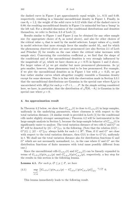
Lemma 4.1. For each p,O≤p≤P, we have
(4.1) sup
θ∈R P
σ>0
�
� � �Gn,θ,σ(·|p)πn,θ,σ(p)−G ∗ n,θ,σ(·|p)π ∗ n,θ,σ(p) � � � � TV
This lemma immediately leads to the following result.
n→∞
−→ 0.