Optimality

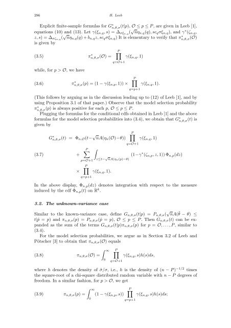
296 H. Leeb
Explicit finite-sample formulas for G∗ n,θ,σ (t|p),O≤p≤P, are given in Leeb [1],
equations (10) and (13). Let γ(ξn,q, s) = ∆σξn,q( √ nηn,q(q), scqσξn,q), and γ∗ (ζn,q,
z, s) = ∆σζn,q( √ nηn,q(q) + bn,qz, scqσξn,q) It is elementary to verify that π∗ n,θ,σ (O)
is given by
(3.5) π ∗ n,θ,σ(O) =
while, for p >O, we have
(3.6)
P�
q=O+1
π ∗ n,θ,σ(p) = (1−γ(ξn,p,1))×
γ(ξn,q,1)
P�
q=p+1
γ(ξn,q,1).
(This follows by arguing as in the discussion leading up to (12) of Leeb [1], and by
using Proposition 3.1 of that paper.) Observe that the model selection probability
π∗ n,θ,σ (p) is always positive for each p,O≤p≤P.
Plugging the formulas for the conditional cdfs obtained in Leeb [1] and the above
formulas for the model selection probabilities into (3.4), we obtain that G∗ n,θ,σ (t) is
given by
(3.7)
G ∗ n,θ,σ(t) = Φn,O(t− √ nA(ηn(O)−θ))
+
×
P�
p=O+1
P�
q=p+1
�
z≤t− √ nA(ηn(p)−θ)
γ(ξn,q,1).
P�
q=O+1
γ(ξn,q,1)
(1−γ ∗ (ζn,p, z,1)) Φn,p(dz)
In the above display, Φn,p(dz) denotes integration with respect to the measure
induced by the cdf Φn,p(t) on R k .
3.2. The unknown-variance case
Similar to the known-variance case, define Gn,θ,σ(t|p) = Pn,θ,σ( √ nA( ˜ θ−θ) ≤
t|ˆp = p) and πn,θ,σ(p) = Pn,θ,σ(ˆp = p),O≤p≤P. Then Gn,θ,σ(t) can be expanded
as the sum of the terms Gn,θ,σ(t|p)πn,θ,σ(p) for p =O, . . . , P, similar to
(3.4).
For the model selection probabilities, we argue as in Section 3.2 of Leeb and
Pötscher [3] to obtain that πn,θ,σ(O) equals
(3.8) πn,θ,σ(O) =
� ∞
0
P�
q=O+1
γ(ξn,q, s)h(s)ds,
where h denotes the density of ˆσ/σ, i.e., h is the density of (n−P) −1/2 times
the square-root of a chi-square distributed random variable with n−P degrees of
freedom. In a similar fashion, for p >O, we get
(3.9) πn,θ,σ(p) =
� ∞
0
(1−γ(ξn,p, s))
P�
q=p+1
γ(ξn,q, s)h(s)ds;