- Page 1 and 2:
Institute of Mathematical Statistic
- Page 3 and 4:
Institute of Mathematical Statistic
- Page 5 and 6:
iv Contents Copulas and Decoupling
- Page 7 and 8:
vi Finally, thanks go the Statistic
- Page 9 and 10:
SCIENTIFIC PROGRAM The Second Erich
- Page 11 and 12:
x Recent Advances in Longitudinal D
- Page 13 and 14:
The Second Lehmann Symposium—Opti
- Page 15 and 16:
xiv Richard Davis Colorado State Un
- Page 17 and 18:
xvi Matthias Matheas Rice Universit
- Page 19 and 20:
xviii Hui Zhao University of Texas
- Page 21 and 22:
IMS Lecture Notes-Monograph Series
- Page 23 and 24:
Proof. The maximum LR test rejects
- Page 25 and 26:
4. Location-scale families On likel
- Page 27 and 28:
6. Conclusions On likelihood ratio
- Page 29 and 30:
IMS Lecture Notes-Monograph Series
- Page 31 and 32:
Student’s t-test for scale mixtur
- Page 33 and 34:
Student’s t-test for scale mixtur
- Page 35 and 36:
Student’s t-test for scale mixtur
- Page 37 and 38:
Optimality in multiple testing 17 w
- Page 39 and 40:
Optimality in multiple testing 19 I
- Page 41 and 42:
power 0.02 0.03 0.04 0.05 0.06 0.07
- Page 43 and 44:
Optimality in multiple testing 23 i
- Page 45 and 46:
Optimality in multiple testing 25 (
- Page 47 and 48:
Optimality in multiple testing 27 M
- Page 49 and 50:
6. Summary Optimality in multiple t
- Page 51 and 52:
Optimality in multiple testing 31 [
- Page 53 and 54:
IMS Lecture Notes-Monograph Series
- Page 55 and 56:
On the false discovery proportion 3
- Page 57 and 58:
On the false discovery proportion 3
- Page 59 and 60:
On the false discovery proportion 3
- Page 61 and 62:
≤ N� � N� P m=1 On the fals
- Page 63 and 64:
Since j≤ s, it follows that On th
- Page 65 and 66:
0.025 0.02 0.015 0.01 0.005 On the
- Page 67 and 68:
On the false discovery proportion 4
- Page 69 and 70:
On the false discovery proportion 4
- Page 71 and 72:
IMS Lecture Notes-Monograph Series
- Page 73 and 74:
Massive multiple hypotheses testing
- Page 75 and 76:
Massive multiple hypotheses testing
- Page 77 and 78:
Massive multiple hypotheses testing
- Page 79 and 80:
Massive multiple hypotheses testing
- Page 81 and 82:
P value EDF qdf 0.0 0.2 0.4 0.6 0.8
- Page 83 and 84:
Massive multiple hypotheses testing
- Page 85 and 86:
Proof. See Appendix. Massive multip
- Page 87 and 88:
X1 Massive multiple hypotheses test
- Page 89 and 90:
Massive multiple hypotheses testing
- Page 91 and 92:
0.0 0.2 0.4 0.6 0.8 1.0 0.0 0.2 0.4
- Page 93 and 94:
Then π0α ∗ cal π0α ∗ cal +
- Page 95 and 96:
Massive multiple hypotheses testing
- Page 97 and 98:
IMS Lecture Notes-Monograph Series
- Page 99 and 100:
Frequentist statistics: theory of i
- Page 101 and 102:
Frequentist statistics: theory of i
- Page 103 and 104:
2.3. Failure and confirmation Frequ
- Page 105 and 106:
3.1. Types of null hypothesis Frequ
- Page 107 and 108:
Frequentist statistics: theory of i
- Page 109 and 110:
Frequentist statistics: theory of i
- Page 111 and 112:
Frequentist statistics: theory of i
- Page 113 and 114:
Frequentist statistics: theory of i
- Page 115 and 116:
Frequentist statistics: theory of i
- Page 117 and 118:
Frequentist statistics: theory of i
- Page 119 and 120:
together with the probabilistic ass
- Page 121 and 122:
Statistical models: problem of spec
- Page 123 and 124:
Statistical models: problem of spec
- Page 125 and 126:
Statistical models: problem of spec
- Page 127 and 128:
Statistical models: problem of spec
- Page 129 and 130:
Statistical models: problem of spec
- Page 131 and 132:
Statistical models: problem of spec
- Page 133 and 134:
Statistical models: problem of spec
- Page 135 and 136:
Statistical models: problem of spec
- Page 137 and 138:
Statistical models: problem of spec
- Page 139 and 140:
Statistical models: problem of spec
- Page 141 and 142:
Modeling inequality, spread in mult
- Page 143 and 144:
Modeling inequality, spread in mult
- Page 145 and 146:
Modeling inequality, spread in mult
- Page 147 and 148:
Modeling inequality, spread in mult
- Page 149 and 150:
Modeling inequality, spread in mult
- Page 151 and 152:
IMS Lecture Notes-Monograph Series
- Page 153 and 154:
Semiparametric transformation model
- Page 155 and 156:
2.1. The model Semiparametric trans
- Page 157 and 158:
Semiparametric transformation model
- Page 159 and 160:
Semiparametric transformation model
- Page 161 and 162:
Semiparametric transformation model
- Page 163 and 164:
Semiparametric transformation model
- Page 165 and 166:
Semiparametric transformation model
- Page 167 and 168:
Semiparametric transformation model
- Page 169 and 170:
Semiparametric transformation model
- Page 171 and 172:
Semiparametric transformation model
- Page 173 and 174:
Semiparametric transformation model
- Page 175 and 176:
Semiparametric transformation model
- Page 177 and 178:
Semiparametric transformation model
- Page 179 and 180:
6.3. Part (ii) Put (6.1) (6.2) ˙Γ
- Page 181 and 182:
Semiparametric transformation model
- Page 183 and 184:
8. Proof of Proposition 2.3 Semipar
- Page 185 and 186:
Semiparametric transformation model
- Page 187 and 188:
Semiparametric transformation model
- Page 189 and 190:
Semiparametric transformation model
- Page 191 and 192:
Bayesian transformation hazard mode
- Page 193 and 194:
Bayesian transformation hazard mode
- Page 195 and 196:
Bayesian transformation hazard mode
- Page 197 and 198:
Cumulative Hazard 0.0 0.2 0.4 0.6 0
- Page 199 and 200:
Hazard function 0.0 0.5 1.0 1.5 2.0
- Page 201 and 202:
Bayesian transformation hazard mode
- Page 203 and 204:
IMS Lecture Notes-Monograph Series
- Page 205 and 206:
Copulas, information, dependence an
- Page 207 and 208:
Copulas, information, dependence an
- Page 209 and 210:
Copulas, information, dependence an
- Page 211 and 212:
Copulas, information, dependence an
- Page 213 and 214:
Copulas, information, dependence an
- Page 215 and 216:
Copulas, information, dependence an
- Page 217 and 218:
Copulas, information, dependence an
- Page 219 and 220:
Copulas, information, dependence an
- Page 221 and 222:
Copulas, information, dependence an
- Page 223 and 224:
Copulas, information, dependence an
- Page 225 and 226:
Copulas, information, dependence an
- Page 227 and 228:
Copulas, information, dependence an
- Page 229 and 230:
Copulas, information, dependence an
- Page 231 and 232:
Regression trees 211 right model in
- Page 233 and 234:
Abs(effects) 0.00 0.05 0.10 0.15 0.
- Page 235 and 236:
Regression trees 215 of the tree. T
- Page 237 and 238:
Regression trees 217 GUIDE methods
- Page 239 and 240:
Regression trees 219 and E appear a
- Page 241 and 242:
Regression trees 221 Table 3 Result
- Page 243 and 244:
Solder =thick 2.5 Regression trees
- Page 245 and 246:
Observed values 0 10 20 30 40 50 60
- Page 247 and 248: Regression trees 227 effects and in
- Page 249 and 250: IMS Lecture Notes-Monograph Series
- Page 251 and 252: On Competing risk and degradation p
- Page 253 and 254: On Competing risk and degradation p
- Page 255 and 256: On Competing risk and degradation p
- Page 257 and 258: On Competing risk and degradation p
- Page 259 and 260: On Competing risk and degradation p
- Page 261 and 262: IMS Lecture Notes-Monograph Series
- Page 263 and 264: Restricted estimation in competing
- Page 265 and 266: Restricted estimation in competing
- Page 267 and 268: Restricted estimation in competing
- Page 269 and 270: Restricted estimation in competing
- Page 271 and 272: 9. Conclusion 0.0 0.1 0.2 0.3 0.4 0
- Page 273 and 274: IMS Lecture Notes-Monograph Series
- Page 275 and 276: 2.1. Maximin efficiency robust test
- Page 277 and 278: Robust tests for genetic associatio
- Page 279 and 280: Robust tests for genetic associatio
- Page 281 and 282: Robust tests for genetic associatio
- Page 283 and 284: Robust tests for genetic associatio
- Page 285 and 286: Robust tests for genetic associatio
- Page 287 and 288: 1 . . . 1 i . . . . . . R j . . . O
- Page 289 and 290: Optimal sampling strategies 269 as
- Page 291 and 292: Optimal sampling strategies 271 γ1
- Page 293 and 294: Optimal sampling strategies 273 Def
- Page 295 and 296: Optimal sampling strategies 275 Usi
- Page 297: Optimal sampling strategies 277 Def
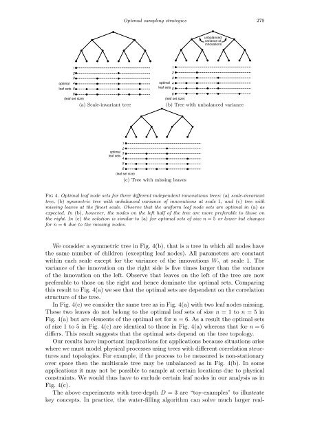
- Page 301 and 302: 6. Related work Optimal sampling st
- Page 303 and 304: Optimal sampling strategies 283 Cla
- Page 305 and 306: Optimal sampling strategies 285 Sin
- Page 307 and 308: Optimal sampling strategies 287 µ
- Page 309 and 310: Optimal sampling strategies 289 on
- Page 311 and 312: IMS Lecture Notes-Monograph Series
- Page 313 and 314: Linear prediction after model selec
- Page 315 and 316: y the P× 1 vector (3.1) ηn(p) = L
- Page 317 and 318: Linear prediction after model selec
- Page 319 and 320: Linear prediction after model selec
- Page 321 and 322: Linear prediction after model selec
- Page 323 and 324: Linear prediction after model selec
- Page 325 and 326: Linear prediction after model selec
- Page 327 and 328: Linear prediction after model selec
- Page 329 and 330: Appendix B: Proofs for Section 5 Li
- Page 331 and 332: Linear prediction after model selec
- Page 333 and 334: Local asymptotic minimax risk/asymm
- Page 335 and 336: Local asymptotic minimax risk/asymm
- Page 337 and 338: Then (3.5) Local asymptotic minimax
- Page 339 and 340: Local asymptotic minimax risk/asymm
- Page 341 and 342: Local asymptotic minimax risk/asymm
- Page 343 and 344: Moment-density estimation 323 may n
- Page 345 and 346: 3. The bias and MSE of ˆf ∗ α M
- Page 347 and 348: Moment-density estimation 327 Corol
- Page 349 and 350:
Moment-density estimation 329 Suppo
- Page 351 and 352:
6. Simulations Moment-density estim
- Page 353 and 354:
Moment-density estimation 333 [7] M
- Page 355 and 356:
for positive α, and for α = 0 as
- Page 357 and 358:
Asymptotics of the MDPDE 337 Lemma
- Page 359:
Asymptotics of the MDPDE 339 asympt