Optimality
Optimality
Optimality
You also want an ePaper? Increase the reach of your titles
YUMPU automatically turns print PDFs into web optimized ePapers that Google loves.
Semiparametric transformation models 151<br />
n −1 � n<br />
i=1 1(Xi ≥ t) and Further, let �·� be the supremum norm in the set<br />
ℓ ∞ ([0, τ]×Θ), and let�·�∞ be the supremum norm ℓ ∞ ([0, τ]). We assume that<br />
the point τ satisfies Condition 2.0(iii).<br />
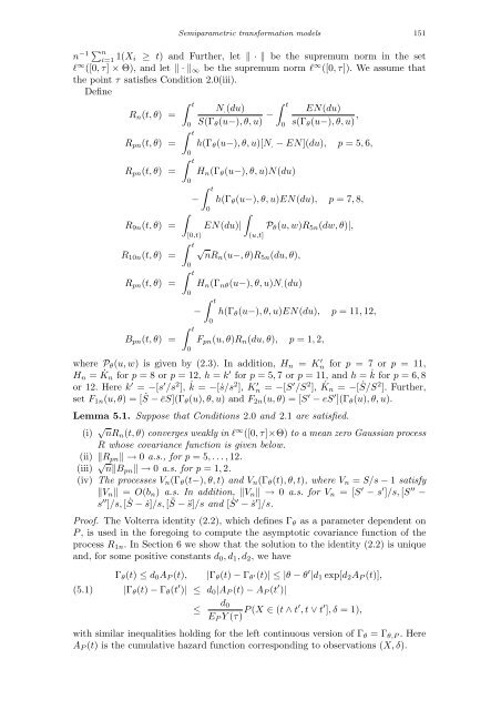
Define<br />
Rn(t, θ) =<br />
Rpn(t, θ) =<br />
Rpn(t, θ) =<br />
R9n(t, θ) =<br />
R10n(t, θ) =<br />
Rpn(t, θ) =<br />
Bpn(t, θ) =<br />
� t<br />
0<br />
� t<br />
0<br />
� t<br />
0<br />
N.(du)<br />
S(Γθ(u−), θ, u) −<br />
� t<br />
EN(du)<br />
0 s(Γθ(u−), θ, u) ,<br />
h(Γθ(u−), θ, u)[N.− EN](du), p = 5,6,<br />
Hn(Γθ(u−), θ, u)N(du)<br />
� t<br />
− h(Γθ(u−), θ, u)EN(du), p = 7, 8,<br />
� 0 �<br />
EN(du)| Pθ(u, w)R5n(dw, θ)|,<br />
[0,t)<br />
� t<br />
0<br />
� t<br />
0<br />
� t<br />
0<br />
(u,t]<br />
√ nRn(u−, θ)R5n(du, θ),<br />
Hn(Γnθ(u−), θ, u)N.(du)<br />
−<br />
� t<br />
0<br />
h(Γθ(u−), θ, u)EN(du), p = 11,12,<br />
Fpn(u, θ)Rn(du, θ), p = 1, 2,<br />
wherePθ(u, w) is given by (2.3). In addition, Hn = K ′ n for p = 7 or p = 11,<br />
Hn = ˙ Kn for p = 8 or p = 12, h = k ′ for p = 5, 7 or p = 11, and h = ˙ k for p = 6, 8<br />
or 12. Here k ′ =−[s ′ /s 2 ], ˙ k =−[˙s/s 2 ], K ′ n =−[S ′ /S 2 ], ˙ Kn =−[ ˙ S/S 2 ]. Further,<br />
set F1n(u, θ) = [ ˙ S− ēS](Γθ(u), θ, u) and F2n(u, θ) = [S ′ − eS ′ ](Γθ(u), θ, u).<br />
Lemma 5.1. Suppose that Conditions 2.0 and 2.1 are satisfied.<br />
(i) √ nRn(t, θ) converges weakly in ℓ ∞ ([0, τ]×Θ) to a mean zero Gaussian process<br />
R whose covariance function is given below.<br />
(ii)�Rpn�→0 a.s., for p = 5, . . . ,12.<br />
(iii) √ n�Bpn�→0 a.s. for p = 1, 2.<br />
(iv) The processes Vn(Γθ(t−), θ, t) and Vn(Γθ(t), θ, t), where Vn = S/s−1 satisfy<br />
�Vn� = O(bn) a.s. In addition,�Vn�→0a.s. for Vn = [S ′ − s ′ ]/s,[S ′′ −<br />
s ′′ ]/s,[ ˙ S− ˙s]/s,[ ¨ S−¨s]/s and [ ˙ S ′ − ˙s ′ ]/s.<br />
Proof. The Volterra identity (2.2), which defines Γθ as a parameter dependent on<br />
P, is used in the foregoing to compute the asymptotic covariance function of the<br />
process R1n. In Section 6 we show that the solution to the identity (2.2) is unique<br />
and, for some positive constants d0, d1, d2, we have<br />
(5.1)<br />
Γθ(t)≤d0AP(t), |Γθ(t)−Γθ ′(t)|≤|θ− θ′ |d1 exp[d2AP(t)],<br />
|Γθ(t)−Γθ(t ′ )| ≤ d0|AP(t)−AP(t ′ )|<br />
≤<br />
d0<br />
EPY (τ) P(X∈ (t∧t′ , t∨t ′ ], δ = 1),<br />
with similar inequalities holding for the left continuous version of Γθ = Γθ,P. Here<br />
AP(t) is the cumulative hazard function corresponding to observations (X, δ).


