Using the Ellipse to Fit and Enclose Data Points ... - Cornell University

Using the Ellipse to Fit and Enclose Data Points
A First Look at Scientific Computing and Numerical
Optimization
Charles F. Van Loan
Department of Computer Science
Cornell University

Problem 1: Ellipse Enclosing
Suppose P a convex polygon with n vertices P1,...,Pn. P1,...,Pn. Findthe
smallest ellipse E that encloses P1,...,Pn.
What do we mean by “smallest”?

Problem 2: Ellipse Fitting
Suppose P a convex polygon with n vertices P1,...,Pn. Find an ellipse E that
is as close as possible to P1,...,Pn.
What do we mean by “close”?

Subtext
Talking about the these problems is a nice way to introduce the field of scientific
computing.
Problems 1 and 2 pose research issues, but we will keep it simple.
We can go quite far towards solving these problems using 1-D minimization
and simple linear least squares.

Outline
• Representation
We consider three possibilities with the ellipse.
• Approximation
We can measure the size of an ellipse by area or perimeter. The latter
is more complicated and requires approximation.
• Dimension
We use heuristics to reduce search space dimension in the enclosure
problem. Sometimes it is better to be approximate and fast than foolproof
and slow.
• Distance
We consider two ways to measure the distance between a point set and
an ellipse, leading to a pair of radically different best-fit algorithms.

Part I. → Representation
Approximation
Dimension
Distance

Representation
In computing, choosing the right representation can simplify your algorithmic
life.
We have several choices when working with the ellipse:
1. The Conic Way
2. The Parametric Way
3. The Foci/String Way

The set of points (x, y) that satisfy
defines an ellipse if
The Conic Way
Ax 2 + Bxy + Cy 2 + Dx + Ey + F =0
B 2 − 4AC < 0.
This rules out hyperbolas like xy +1=0and3x 2 − 2y 2 +1=0.
This rules out parabolas like x 2 + y =0and−3y 2 + x +2=0.
To avoid degenerate ellipses like 3x 2 +4y 2 + 1 = 0 we also require
D 2
4A
+ E2
4C
− F>0

The Conic Way (Cont’d)
Without loss of generality we may assume that A =1.
An ellipse is the set of points (x, y) thatsatisfy
subject to the constraints
and
x 2 + Bxy + Cy 2 + Dx + Ey + F =0
D 2
An ellipse has five parameters.
4
B 2 − 4C 0

The Parametric Way
This is an ellipse with center (h, k) and semiaxes a and b:
⎛
⎜
⎝
x − h
a
i.e., the set of points (x(t),y(t)) where
and 0 ≤ t ≤ 2π.
Where is the fifth parameter?
⎞
⎟
⎠
2
+
⎛
⎜
⎝
y − k
b
⎞
⎟
⎠
x(t) =h + a cos(t)
y(t) = k + b sin(t)
2
= 1

The Parametric Way (Cont’d)
The tilt of the ellipse is the fifth parameter.
Rotate the ellipse counter-clockwise by τ radians:
In matrix-vector notation:
x(t) =h +cos(τ)[a cos(t)] − sin(τ)[b sin(t)]
y(t) = k +sin(τ)[a cos(t)] + cos(τ)[b sin(t)]
⎡
⎢
⎣
x(t)
y(t)
⎤
⎥
⎦ =
⎡
⎢
⎣
h
k
⎤
⎥
⎦ +
⎡
⎢
⎣
cos(τ) − sin(τ)
sin(τ) cos(τ)
⎤ ⎡
⎥ ⎢
⎥ ⎢
⎥ ⎢
⎥ ⎢
⎦ ⎣
a cos(t)
b sin(t)
⎤
⎥
⎦

Example 1: No tilt and centered at (0,0)
6
4
2
0
−2
−4
−6
⎡
⎢
⎣
x(t)
y(t)
⎤
⎥
⎦ =
⎡
⎢
⎣
5cos(t)
3sin(t)
a = 5, b = 3, (h,k) = (0,0), tau = 0 degrees
−8 −6 −4 −2 0 2 4 6 8
⎤
⎥
⎦
focii

Example 2. 30 o tilt and centered at (0,0)
⎡
⎢
⎣
x(t)
y(t)
6
4
2
0
−2
−4
−6
⎤
⎥
⎦ =
⎡
⎢
⎣
cos(30 o ) − sin(30 o )
sin(30 o ) cos(30 o )
a = 5, b = 3, (h,k) = (0,0), tau = 30 degrees
⎤ ⎡
⎥ ⎢
⎥ ⎢
⎥ ⎢
⎥ ⎢
⎦ ⎣
focii
5cos(t)
3sin(t)
−8 −6 −4 −2 0 2 4 6 8
⎤
⎥
⎦

Example 3. 30 o tilt and centered at (2,1)
⎡
⎢
⎣
x(t)
y(t)
⎤
⎥
⎦ =
6
4
2
0
−2
−4
−6
⎡
⎢
⎣
2
1
⎤
⎥
⎦ +
⎡
⎢
⎣
cos(30 o ) − sin(30 o )
sin(30 o ) cos(30 o )
a = 5, b = 3, (h,k) = (2,1), tau = 30 degrees
focii
⎤ ⎡
⎥ ⎢
⎥ ⎢
⎥ ⎢
⎥ ⎢
⎦ ⎣
−8 −6 −4 −2 0 2 4 6 8
5cos(t)
3sin(t)
⎤
⎥
⎦

The Foci/String Way
Suppose points F1 =(x1,y1)andF2 =(x2,y2) are given and that s is a positive
number greater than the distance between them.
The set of points (x, y) that satisfy
defines an ellipse.
�
(x − x1) 2 +(y − y1) 2 + �
(x − x2) 2 +(y − y2) 2 = s
The points F1 and F2 are the foci of the ellipse.
The sum of the distances to the foci is a constant designated by s and from the
“construction” point of view can be thought of as the “string length.”

The Foci/String Way (Cont’d)
F 1
5.32 2.68
s = 8.00
Ellipse Construction: Anchor a piece of string with length s at the two
foci. With your pencil circumnavigate the foci always pushing out against
the string.
F 2

Conversions: Conic −→ Parametric
If Ax 2 + Bxy + Cy 2 + Dx + Ey + F = 0 specifies an ellipse and we define the
matrices
then
M0 =
⎡
⎢
⎣
F D/2E/2 D/2 A B/2
E/2 B/2 C
⎤
⎥
⎦
M =
⎡
⎢
⎣
A B/2
B/2 C
a = �
−det(M0)/(det(M)λ1) b = �
−det(M0)/(det(M)λ2)
h =(BE − 2CD)/(4AC − B 2 ) k =(BD − 2AE)/(4AC − B 2 )
τ = arccot((A − C)/B)/2
where λ1 and λ2 are the eigenvalues of M ordered so that |λ1 − A| ≤|λ1 − C|.
(This ensures that |λ2 − C| ≤|λ2 − A|.)
⎤
⎥
⎦

Conversions: Parametric −→ Conic
If c =cos(τ) ands =sin(τ), then the ellipse
x(t) =h + c [ a cos(t)] − s [ b sin(t)]
y(t) = k + c [ a cos(t)] + c [ b sin(t)]
is also specified by Ax 2 + Bxy + Cy 2 + Dx + Ey + F = 0 where
A =(bc) 2 +(as) 2
B = −2cs(a 2 − b 2 )
C =(bs) 2 +(ac) 2
D = −2Ah − kB
E = −2Ck − hB
F = −(ab) 2 + Ah 2 + Bhk + Ck 2

Conversions: Parametric −→ Foci/String
Let E be the ellipse
x(t) =h +cos(τ)[a cos(t)] − sin(τ)[b sin(t)]
y(t) = k +sin(τ)[a cos(t)] + cos(τ)[b sin(t)]
If c = √ a 2 − b 2 then E has foci
F1 =(h − cos(τ)c, k − sin(τ)c) F2 =(h +cos(τ)c, k +sin(τ)c)
and string length
s =2a

Conversions: Foci/String −→ Parametric
If F1 =(α1,β1), F2 =(α2,β2), and s defines an ellipse, then
a = s/2
b = �
s 2 − ((α1 − α2) 2 +(β1 − β2) 2 )) / 2
h =(α1 + α2)/2
k =(β1 + β2)/2
τ = arctan((β2 − β1)/(α2 − α1))

Summary of the Representations
Parametric: h , k, a, b, andτ.
E =
⎧
⎪⎨
⎪⎩
(x, y)
� ⎡
�
�
� ⎢
� ⎢
� ⎢
� ⎢
� ⎣
�
�
x
y
⎤
⎥
⎦ =
Conic: B, C, D, E, andF
E = �
⎡
⎢
⎣
h
k
⎤
⎥
⎦ +
⎡
⎢
⎣
cos(τ) − sin(τ)
sin(τ) cos(τ)
⎤ ⎡
⎥ ⎢
⎥ ⎢
⎥ ⎢
⎥ ⎢
⎦ ⎣
a cos(t)
b sin(t)
(x, y) | x 2 + Bxy + Cy 2 + Dx + Ey + F =0 �
Foci/String: α1, β1, α2, β2, ands.
E = �
(x, y) � � ���
⎤
⎥
⎦
, 0 ≤ t ≤ 2π
�
(x − α1) 2 +(y − β1) 2 + �
(x − α2) 2 +(y − β2) 2 = s. �
⎫
⎪⎬
⎪⎭

Representation
Part II. → Approximation
Dimension
Distance

The Size of an Ellipse
How big is an ellipse E with semiaxes a and b?
Two reasonable metrics:
Area(E) =πab
Perimeter(E) = � 2π
0
�
(a sin(t)) 2 +(b cos(t)) 2 ) dt
There is no simple closed-form expression for the perimeter of an ellipse.
To compute perimeter we must resort to approximation.

Some Formulas for Perimeter Approximation
Perimeter(E) ≈
⎧
⎪⎨
⎪⎩
π (a + b)
π(a + b) · 3 − √ 1 − h
2
π(a + b) · (1 + h/8) 2
π(a + b) · (3 − √ 4 − h)
π(a + b) ·
π(a + b) · (1 +
π(a + b) ·
π �
�
�
2(a 2 + b 2 )
64 − 3h2
64 − 16h
3h
10 + √ 4 − 3h )
256 − 48h − 21h2
256 − 112h +3h 2
�
�
� π 2(a2 + b2 (a − b)
) − 2
2
h =
⎛
⎜
⎝
a − b
a + b
⎞
⎟
⎠
2
(1)
(2)
(3)
(4)
(5)
(6)
(7)
(8)
(9)

Relative Error as a Function of Eccentricity
e =
�
�
�
�
�
�
Relative Error
10 0
10 −2
10 −4
10 −6
10 −8
10 −10
10 −12
10 −14
(1)
(8)
(3)
(6)
(5)
10
0 0.1 0.2 0.3 0.4 0.5 0.6 0.7 0.8 0.9
−16
e = Eccentricity
�1 −
⎛
⎜
⎝
b
a
⎞
⎟
⎠
2
e =0⇒ circle, e = .99 ⇒ cigarlike

Apply a quadrature rule to
For example:
Perimeter via Quadrature
Perimeter(E) = � 2π
0
�
(a sin(t)) 2 +(b cos(t)) 2 ) dt
function P = Perimeter(a,b,N)
% Rectangle rule with N rectangles
t = linspace(0,2*pi,N+1);
h = 2*pi/N;
P = h*sum(sqrt((a*cos(t)).^2 + (b*sin(t)).^2));
How do you chose N?
What is the error?

Efficiency and Accuracy
Compared to a formula like π(a+b), the function Perimeter(a,b,N) is much
more expensive to evaluate.
The relative error of Perimeter(a,b,N) is about O(1/N 2 ).
Can we devise an approximation with an easily computed rigorous error bound?

Computable Error Bounds
For given n, define inner and outer polygons by the points
(a cos(kδ),bsin(kδ) fork =0:n − 1andδ =2π/n.
⎛
⎜
⎝
Inner Polygon
Perimeter
⎞
⎟
⎠ ≤ Perimeter(E) ≤
⎛
⎜
⎝
Outer Polygon
Perimeter
⎞
⎟
⎠

Relative Error as a Function of n
e n =10 n =10 2 n =10 3 n =10 4 n =10 5 n =10 6
0.00 1.590 · 10 −1 1.551 · 10 −3 1.550 · 10 −5 1.550 · 10 −7 1.555 · 10 −9 1.114 · 10 −11
0.50 1.486 · 10 −1 1.449 · 10 −3 1.448 · 10 −5 1.448 · 10 −7 1.448 · 10 −9 1.461 · 10 −11
0.90 1.164 · 10 −1 1.157 · 10 −3 1.156 · 10 −5 1.156 · 10 −7 1.156 · 10 −9 1.163 · 10 −11
0.99 6.755 · 10 −2 1.015 · 10 −3 1.015 · 10 −5 1.015 · 10 −7 1.015 · 10 −9 1.003 · 10 −11
e = eccentrity =
Error mildly decreases with eccentricity.
�
�
�
�
�
�
�1 −
⎛
⎜
⎝
b
a
⎞
⎟
⎠
2

Summary of the Area vs. Perimeter Issue
The “inverse” of the enclosing ellipse problem is the problem of inscribing the
largest possible polygon in an ellipse.
Max Area Vertices
Max Perimeter Vertices
The choice of objective function, Area(E) or Perimeter(E), matters. For the
enclosing ellipse problem we will have to make a choice.

Representation
Approximation
Part III. → Dimension
Distance

Enclosing Data with an Ellipse
Given a point set P = { (x1,y1), ..., (xn,yn)}, minimize Area(E) subject
to the constraint that E encloses P.
Everything that follows could be adapted if we used Perimeter(E).

Simplification: Convex Hull
The ConvHull(P) is a subset of P which when connected in the right order
define a convex polyon that encloses P.
The minimum enclosing ellipse for ConvHull(P) is the same as the minimum
enclosing ellipse for P. This greatly reduces the “size” of the problem.

Is the point (x, y) inside the ellipse E?
Checking Enclosure
Compute the distances to the foci F1 =(α1,β1)andF2 =(α2,β2) and compare
the sum with the string length s.
In other words, if
�
(x − β1) 2 +(y − β1) 2 + �
(x − α2) 2 +(y − β2) 2 ≤ s
then (x, y) isinsideE.

The “Best” E given Foci F1 and F2
If F1 =(α1,β1)andF2 =(α2,β2) are fixed, then area is a function of the string
length s. In particular, if
then it can be shown that
d = �
(α1 − α2) 2 +(β1 − β2) 2
Area(E) = π s
4
√ s 2 − d 2
If E is to enclose P = { (x1,y1), ...,(xn,yn)}, and have minimal area, we
want the smallest possible s, i.e.,
s(F1,F2) = max
1 ≤ i ≤ n
�
(xi − α1) 2 +(yi − β1) 2 + �
(xi − α2) 2 +(yi − β2) 2

The “Best” E given Foci F1 and F2 (Cont’d)
Locate the point whose distance sum to the two foci is maximal. This determines
sopt and Eopt
Area(Eopt) = π
4 sopt
�
�
�
�
⎛
�
�
�
⎝ sopt
2
⎞
⎠
2
−
⎛
⎜
⎝
d
2
⎞
⎟
⎠
2

The “Best” E given Center (h, k) and Tilt τ
Foci location depends on the space between them d:
F1(d) =
F2(d) =
⎛
⎝h − d 2 cos(τ) ,k− d 2 sin(τ)
⎛
⎝h + d 2 cos(τ) ,k+ d 2 sin(τ)
Optimum string length s(F1(d),F2(d)) is also a function of d
The minimum area enclosing ellipse with center (h, k) and tilt τ, is defined by
setting d = d∗ where d∗ minimizes
fh,k,τ(d) = π s
4
√ s 2 − d 2 s = s(F1(d),F2(d))
⎞
⎠
⎞
⎠

The “Best” E given Center (h, k) and Tilt τ (Cont’d)
For each choice of separation d along the tilt line, we get a different minimum
enclosing ellipse. Finding the best d is a Golden Section Search problem.

The “Best” E given Center (h, k) and Tilt τ (Cont’d)
Typical plot of the function
fh,k,τ(d) = π s
4
√ s 2 − d 2 s = s(F1(d),F2(d))
for d ranging from 0 to max { �
(x(i) − h) 2 +(y(i) − k) 2 }:
8.5
8
7.5
7
6.5
6
0 0.5 1 1.5

Heuristic Choice for Center(h, k) and Tilt τ
Assume that (xp,yp) and(xq,yq) are the two points in P that are furthest
apart. (They specify the diameter of P.)
Instead of looking for the optimum h, k, andτ we can set
h = xp + xq
2
k = yp + yq
2
τ = arctan ⎝ yq − yp
⎛
xq − xp
and then complete the specification of an approximately optimum E by determining
d∗ and s(F1(d∗),F2(d∗)) as above.
We’ll call this the hkτ-heuristic approach. Idea: the major axis tends to be
along the line where the points are dispersed the most.
⎞
⎠

The “Best” E given Center (h, k)
The optimizing d∗ for the function fh,k,d(d) depends on the tilt parameter τ.
Denote this dependence by d∗(τ) .
The minimum-area enclosing ellipse with center (h, k) is defined by setting
τ = τ∗ where τ∗ minimizes
˜fh,k(τ) = π s
4
�
s 2 − d∗(τ) 2 s = s(F1(d∗(τ)),F2(d∗(τ)))

The “Best” E given Center (h, k) (Cont’d)
Typical plot of the function
˜fh,k(τ) = π s �
s
4
2 − d∗(τ) 2 s = s(F1(d∗(τ)),F2(d∗(τ)))
across the interval 0 ≤ τ ≤ 360o :
Area
4
3.5
3
2.5
2
1.5
1
0.5
0
0 50 100 150 200 250 300 350
tau

The “Best” E
The optimizing τ∗ for the function ˜ fh,k(τ) depends on the center coordinates h
and k.
Denote this dependence by τ∗(h, k)) .
The minimum-area enclosing ellipse is defined by setting (h, k) =(h∗,k∗) where
h∗ and k∗ minimize
where
F (h, k) = ˜ fh,k(τ∗(h, k)) = π s
4
�
s 2 − d∗(τ∗(h, k)) 2
s = s(F1(d∗(τ∗(h, k))),F2(d∗(τ∗(h, k))))

The “Best” E
Through these devices we have reduced to two the dimension of the search for
the minimum area enclosing ellipse.

Representation
Approximation
Dimension
Part IV. → Distance

Approximating Data with an Ellipse
We need to define the distance from a point set P = {P1,...,Pn} to an ellipse
E.

The Point set P:
The Ellipse E:
The distance from P to E:
Goodness-of-Fit: Conic Residual
dist(P, E) = n �
{ (α1,β1),...,(αn,βn) }
x 2 + Bxy + Cy 2 + Dx + Ey + F = 0
i=1
�
α 2 i + αiβiB + β 2 i C + αiD + βiE + F � 2
Sum the squares of what’s “left over” when you plug each (αi,βi) into the
ellipse equation.

A Linear Least Squares Problem with Five
Unknowns
dist(P, E) =
�
�
�
�
�
�
�
�
�
�
�
�
�
�
�
�
�
�
�
�
�
�
�
�
�
�
�
�
�
�
�
�
�
�
⎡
⎢
⎣
α1β1 β2 1 α1 β1 1
α2β2 β2 2 α2 β2 1
α3β3 β2 3 α3 β3 1
. . . . .
αn−1βn−1 β2 n−1 αn−1 βn−1 1
αnβn β2 n αn βn 1
⎤
⎥ ⎡
⎥ ⎢
⎥ ⎢
⎥ ⎢
⎥ ⎢
⎥ ⎢
⎥ ⎢
⎥ ⎢
⎥ ⎢
⎥ ⎢
⎥ ⎢
⎥ ⎢
⎥ ⎢
⎥ ⎢
⎥ ⎢
⎥ ⎢
⎥ ⎢
⎥ ⎢
⎥ ⎢
⎥ ⎢
⎥ ⎣
⎥
⎦
B
C
D
E
F
⎤
⎥
⎦
+
⎡
⎢
⎣
α1
α2
α3
.
αn−1
αn
⎤
⎥
⎦
�
�
�
�
�
�
�
�
�
�
�
�
�
�
�
�
�
�
�
�
�
�
�
�
�
�
�
�
�
�
�
�
�
�
2
2

The Point set P:
The Ellipse E:
The distance from P to E:
Goodness-of-Fit: Point Proximity
{ (α1,β1),...,(αn,βn) }
x(t) =h +cos(τ)[a cos(t)] − sin(τ)[b sin(t)]
y(t) = k +sin(τ)[a cos(t)] + cos(τ)[b sin(t)]
dist(P, E) = n �
i=1 ((x(ti) − αi) 2 +(y(ti) − βi) 2
where (x(ti),y(ti)) is the closest point on E to (αi,βi), i =1:n.

Distance from a Point to an Ellipse
Let E be the ellipse
x(t) =h +cos(τ)[a cos(t)] − sin(τ)[b sin(t)]
y(t) = k +sin(τ)[a cos(t)] + cos(τ)[b sin(t)]
To find the distance from point P =(α, β) toE define
and set
d(t) = �
(α − x(t)) 2 +(β − y(t)) 2
dist(P, E) = min
0 ≤ t ≤ 2π
Note that d(t) is a function of a single variable.
d(t)

6
5
4
3
2
1
0
−1
−2
“Drop” Perpendiculars
−4 −3 −2 −1 0 1 2 3 4 5 6
The nearest point on the ellipse E is in the same “ellipse quadrant”.

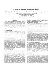
Comparison: Conic Residual vs Point Proximity
The two methods render different best-fitting ellipses.
Conic Residual method is much faster but it may render a hyperbola if the data
is “bad”.

Conic Residual Method w/o Constraints
3
2.5
2
1.5
1
0.5
0
−0.5
−1
−1.5
−2
0 2 4 6 8 10
There are fast ways to solve the conic residual least squares problem with the
constraint C>B 2 /4 which forces the solution
to define an ellipse.
x 2 + Bxy + Cy 2 + Dx + Ey + F =0

Overall Conclusions
• Representation
The Parametric Representation if not “friendly” when you want to
check if a point is inside an ellipse. The Conic representation led to a
very simple algorithm for the best-fit problem.
• Approximation
There are many ways to approximate the perimeter of an ellipse. Although
we defined the size of an ellipse in terms of its easily-computed
area, it would also be possible to work with perimeter.
• Dimension
We use heuristics to reduce search space dimension in the enclosure
problem.
• Distance
We consider two ways to measure the distance between a point set and
an ellipse, leading to a pair of radically different best-fit algorithms.