de Casteljau's algorithm General formula ∑ Bernstein polynomials
de Casteljau's algorithm General formula ∑ Bernstein polynomials
de Casteljau's algorithm General formula ∑ Bernstein polynomials

Create successful ePaper yourself
Turn your PDF publications into a flip-book with our unique Google optimized e-Paper software.
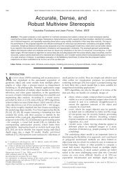
Curves<br />
• So far we’ve seen polylines<br />
• GL_LINE_STRIP, etc.<br />
• Smooth curves would be better for<br />
• building mo<strong>de</strong>ls<br />
• animation<br />
• Possible representations<br />
• Explicit y=f (x)<br />
• can use only if the curve is a function<br />
• Implicit f (x,y,z) = 0<br />
• difficult to work with<br />
• Parametric (f (u), g(u))<br />
Function Not a function!<br />
• Our choice: parametric curves where the functions<br />
n<br />
are all <strong>polynomials</strong> in the parameter x(<br />
u)<br />
=<br />
• easy (and efficient) to compute<br />
<strong>∑</strong>ak<br />
k=<br />
0<br />
• infinitely differentiable<br />
• we’ll look at ones <strong>de</strong>fined by control points<br />
n<br />
k<br />
y(<br />
u)<br />
=<br />
and an <strong>algorithm</strong> operating on them<br />
<strong>∑</strong>bku<br />
52438S Computer Graphics Winter 2004 1<br />
k=<br />
0<br />
Kari Pulli<br />
V ′ =<br />
0<br />
V ′ =<br />
1<br />
V ′<br />
=<br />
0<br />
=<br />
=<br />
B(<br />
u)<br />
=<br />
( 1−<br />
u)<br />
( 1−<br />
u)<br />
K<br />
<strong>General</strong> <strong>formula</strong><br />
( 1−<br />
u)<br />
V ′ 0 + uV<br />
′ 1<br />
( 1−<br />
u)<br />
( ( 1−<br />
u)<br />
V0<br />
+ uV1<br />
) + u(<br />
( 1−<br />
u)<br />
V1<br />
+ uV2<br />
)<br />
2 ( 1−<br />
u)<br />
V + 2(<br />
1−<br />
u)<br />
uV<br />
2<br />
+ u V<br />
K<br />
n<br />
<strong>∑</strong><br />
k<br />
V<br />
⎛n<br />
⎞<br />
⎜ ⎟<br />
⎝k<br />
⎠<br />
0<br />
+ uV<br />
V + uV<br />
1<br />
0<br />
1<br />
2<br />
( n−k<br />
) k ( 1−<br />
u)<br />
u Vk<br />
1<br />
52438S Computer Graphics Winter 2004 3<br />
Kari Pulli<br />
2<br />
binomial coefficient<br />
1 3 3 1<br />
1 4<br />
1<br />
11<br />
1 2 1<br />
1 51010<br />
5<br />
u<br />
6 4 1<br />
1<br />
k<br />
Pascal's<br />
triangle<br />
⎛n<br />
⎞ n!<br />
⎜ ⎟ =<br />
⎝k<br />
⎠ k!<br />
( n − k)!<br />
V0<br />
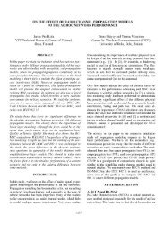
Bézier curve: <strong>de</strong> Casteljau’s<br />
<strong>algorithm</strong><br />
• Evaluate point B(u) by recursive linear interpolation<br />
V1 V’1<br />
V”1<br />
V2<br />
V’2<br />
V’0 = (1-u) V0 + u V1<br />
V’1 = (1-u) V1 + u V2<br />
V’2 = (1-u) V2 + u V3<br />
V”0 = (1-u) V’0 + u V’1<br />
= (1-u) ((1-u)V0+uV1) + u((1-u)V1+uV2)<br />
= (1-u)<br />
V’0<br />
V”0<br />
V3<br />
• What if u=0? u=1?<br />
• What’s the relationship between the number of control points<br />
and the <strong>de</strong>gree of the <strong>polynomials</strong>?<br />
2 V0 + 2(1-u)uV1 + u2 V2<br />
V”1 = (1-u) V’1 + u V’2<br />
= (1-u) ((1-u)V1+uV2) + u((1-u)V2+uV3)<br />
= (1-u) 2 V1 + 2(1-u)uV2 + u2 V”’0<br />
V3<br />
V”’0 = (1-u) V”0 + u V”1<br />
= ...<br />
= (1-u) 3V0 + 3(1-u) 2uV1 + 3(1-u)u2V2 + u3 How much is u?<br />
V'0 divi<strong>de</strong>s V0-V1 1:3<br />
so 3 parts V0 and<br />
1 part V1 so<br />
0.75 V0 + 0.25 V1<br />
V3<br />
u=0 => V0, u=1 => V3, so interpolates endpoints<br />
Degree of polynomial one less than # controls<br />
52438S Computer Graphics Winter 2004 2<br />
Kari Pulli<br />
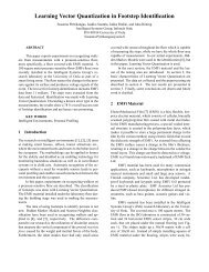
<strong>Bernstein</strong> <strong>polynomials</strong><br />
• The coefficients of the control<br />
points are functions called<br />
the <strong>Bernstein</strong> <strong>polynomials</strong><br />
3<br />
B0<br />
( u)<br />
= ( 1−<br />
u)<br />
2<br />
B1<br />
( u)<br />
= 3u(<br />
1−<br />
u)<br />
2<br />
B2<br />
( u)<br />
= 3u<br />
( 1−<br />
u)<br />
3<br />
B ( u)<br />
= u<br />
• Useful properties (when 0
Bezier Java applet<br />
• Try this online at<br />
http://www.gris.uni-tuebingen.<strong>de</strong>/projects/ilo/repository/bezier.jar<br />
• Move the<br />
• interpolation point, see how the others (and the point on<br />
curve) move<br />
• control points (can even make loops)<br />
52438S Computer Graphics Winter 2004 5<br />
Kari Pulli<br />
V0<br />
V0 '<br />
V1<br />
V0 "<br />
Subdivi<strong>de</strong> and conquer<br />
V1 '<br />
Q(u)<br />
L = [V0,V’0,V”0,V”’0]<br />
R = [V”’0,V”1,V’2,V3]<br />
evaluated at u=0.5<br />
note: V”’0 = Q(0.5)<br />
V1 "<br />
V2<br />
V2 '<br />
52438S Computer Graphics Winter 2004 7<br />
Kari Pulli<br />
V3<br />
<strong>de</strong>f DisplayBezier(V):<br />
if FlatEnough(V):<br />
Line(V[0],V[3])<br />
else:<br />
L,R = Subdivi<strong>de</strong>(V)<br />
DisplayBezier(L)<br />
DisplayBezier(R)<br />
Displaying Bézier curves<br />
• How could we draw<br />
one of these things?<br />
• It would be nice if we<br />
had an adaptive<br />
<strong>algorithm</strong>, that would<br />
take into account<br />
curvature / flatness<br />
V0<br />
<strong>de</strong>f DisplayBezier(V):<br />
assert(len(V) == 4)<br />
if FlatEnough(V):<br />
Line(V[0],V[3])<br />
else:<br />
something<br />
52438S Computer Graphics Winter 2004 6<br />
Kari Pulli<br />
Testing for flatness<br />
V0<br />
• Compare total length of control polygon to length of<br />
line connecting endpoints:<br />
0<br />
52438S Computer Graphics Winter 2004 8<br />
Kari Pulli<br />
V1<br />
3<br />
V1<br />
V2<br />
V0<br />
−V1<br />
+ V1<br />
−V2<br />
+ V2<br />
−V3<br />
< 1+<br />
ε<br />
V −V<br />
V2<br />
V3<br />
V3
More complex curves<br />
• Suppose we want to draw a more complex curve<br />
Why not use a high-or<strong>de</strong>r Bézier?<br />
High or<strong>de</strong>r <strong>polynomials</strong> are difficult to control<br />
• Instead, we’ll splice together a curve from individual<br />
segments that are cubic Béziers<br />
Why cubic?<br />
Lowest dimension with control for the second <strong>de</strong>rivative<br />
Lowest dimension for non-planar polynomial curves<br />
• There are three properties we’d like to have in our<br />
newly constructed splines…<br />
52438S Computer Graphics Winter 2004 9<br />
Kari Pulli<br />
Interpolation<br />
• Bézier curves are<br />
approximating<br />
• The curve does not<br />
(necessarily) pass through all<br />
the control points<br />
• Each point pulls the curve<br />
toward it, but other points are<br />
pulling as well<br />
• Instead, we may prefer a<br />
spline that is interpolating<br />
• That is, that always passes<br />
through every control point<br />
52438S Computer Graphics Winter 2004 11<br />
Kari Pulli<br />
• Every control point affects<br />
every point on the curve<br />
(except the endpoints)<br />
• Moving a single control<br />
point affects the whole<br />
curve!<br />
Local control<br />
• We’d like our spline to have local control<br />
• that is, have each control point affect some well-<strong>de</strong>fined<br />
neighborhood around that point<br />
52438S Computer Graphics Winter 2004 10<br />
Kari Pulli<br />
C 1 only<br />
Continuity<br />
• We want our curve to have continuity<br />
• There shouldn’t be an abrupt change when we move from<br />
one segment to the next.<br />
• There are nested <strong>de</strong>grees of continuity:<br />
Not C0 : C0 :<br />
C 1 ,C 2 : C 3 , C 4 , …:<br />
Superscript tells how many <strong>de</strong>rivatives<br />
are continuous<br />
C<br />
52438S Computer Graphics Winter 2004 12<br />
Kari Pulli<br />
2
Ensuring continuity<br />
• C2 continuous curves would be nice<br />
• Since the functions <strong>de</strong>fining a Bézier curve are<br />
polynomial<br />
• all their <strong>de</strong>rivatives exist and are continuous<br />
• therefore, we only need to worry about the <strong>de</strong>rivatives at the<br />
endpoints of the curve<br />
3 ⎛ 3⎞<br />
( 3−k<br />
) k<br />
B(<br />
u)<br />
= <strong>∑</strong>⎜<br />
⎟(<br />
1−<br />
u)<br />
u Vk<br />
k ⎝k<br />
⎠<br />
3<br />
= 1− u V<br />
2<br />
2<br />
+ 3 1−<br />
u uV + 3 1−<br />
u u V<br />
3<br />
+ u V<br />
=<br />
( ) 0 ( ) 1 ( ) 2 3<br />
2 3<br />
2 3<br />
2 3<br />
3<br />
( 1− 3u<br />
+ 3u<br />
− u ) V + 3(<br />
u − 2u<br />
+ u ) V1<br />
+ 3(<br />
u − u ) V2<br />
+ u V3<br />
3 ⎡−<br />
u<br />
⎢ 2<br />
⎢ 3u<br />
=<br />
⎢−<br />
3u<br />
⎢<br />
⎣ 1<br />
3u<br />
− 6u<br />
3<br />
2<br />
3u<br />
0<br />
0<br />
3<br />
− 3u<br />
3u<br />
2<br />
0<br />
0<br />
3<br />
u ⎤ ⎡V0<br />
⎤<br />
⎥ ⎢ ⎥<br />
0⎥<br />
⎢<br />
V1<br />
⎥ = u<br />
0⎥<br />
⎢V<br />
⎥ 2<br />
⎥ ⎢ ⎥<br />
0⎥⎦<br />
⎣V<br />
⎦<br />
3 2 [ u u 1]<br />
⎡ −1<br />
⎢<br />
⎢<br />
3<br />
⎢−<br />
3<br />
⎢<br />
⎣ 1<br />
1⎤<br />
⎡V0<br />
⎤<br />
0<br />
⎥ ⎢ ⎥<br />
⎢<br />
V<br />
⎥ 1 ⎥<br />
0⎥<br />
⎢V<br />
⎥ 2<br />
⎥ ⎢ ⎥<br />
0⎦<br />
⎣V<br />
⎦<br />
3<br />
3<br />
52438S Computer Graphics Winter 2004 13<br />
Kari Pulli<br />
52438S Computer Graphics Winter 2004 15<br />
Kari Pulli<br />
3<br />
− 6<br />
Derivatives at the endpoints<br />
B′<br />
( 0)<br />
= 3(<br />
V −V<br />
B′<br />
( 1)<br />
= 3(<br />
V −V<br />
B′<br />
′ ( 0)<br />
= 6(<br />
V − 2V<br />
+ V<br />
1<br />
3<br />
0<br />
B′<br />
′ ( 1)<br />
= 6(<br />
V − 2V<br />
+ V )<br />
1<br />
0<br />
2<br />
)<br />
)<br />
1<br />
2<br />
2<br />
3<br />
)<br />
V0<br />
• In general, the nth <strong>de</strong>rivative at an endpoint <strong>de</strong>pends<br />
only on the n+1 points nearest that endpoint<br />
• Geometrical interpretation of <strong>de</strong>rivatives?<br />
1 st <strong>de</strong>rivative at start 3 times the vector V1 –V0 (V3 –V2 at the end)<br />
2 nd <strong>de</strong>rivative 6 times the vector sum of V0 –V1 and V2 –V1<br />
V1<br />
V2<br />
3<br />
0<br />
− 3<br />
3<br />
0<br />
0<br />
V3<br />
• B''(1)?<br />
Evaluating <strong>de</strong>rivatives<br />
3<br />
B(<br />
u)<br />
= [ u<br />
2<br />
u u<br />
⎡ −1<br />
⎢<br />
] ⎢<br />
3<br />
1<br />
⎢−<br />
3<br />
⎢<br />
⎣ 1<br />
• How do we get <strong>de</strong>rivatives<br />
w.r.t u?<br />
• What is B'(0)? ⎡ −1<br />
3 − 3 1⎤<br />
⎢<br />
3 − 6<br />
⎢−<br />
3<br />
⎢<br />
⎣ 1<br />
3<br />
0<br />
3 0<br />
⎥<br />
0 0⎥<br />
⎥<br />
0 0⎦<br />
− 6<br />
[ 0 0 1 0]<br />
⎢<br />
⎥ = [ − 3 3 0 0]<br />
− 3<br />
1⎤<br />
⎡V0<br />
⎤<br />
0<br />
⎥ ⎢ ⎥<br />
⎥ ⎢<br />
V1<br />
⎥<br />
0⎥<br />
⎢V<br />
⎥ 2<br />
⎥ ⎢ ⎥<br />
0⎦<br />
⎣V3<br />
⎦<br />
52438S Computer Graphics Winter 2004 14<br />
Kari Pulli<br />
3<br />
3<br />
0<br />
3<br />
0<br />
0<br />
Just differentiate [u 3 u 2 u 1]<br />
[3u2 2u 1 0](u=0) =[0 0 1 0]<br />
=> -3V0 + 3V1<br />
[6u 2 0 0](u=1) =[6 2 0 0]<br />
=> 6V1 - 12V2 + 6V3<br />
Ensuring C 2 continuity<br />
• Given a cubic Bézier segment (V0,V1,V2,V3)<br />
• add another curve (W0,W1,W2,W3) to it<br />
• in such a way that the joint is C 2<br />
• But first, if a and b are points, what is (2a-b)?<br />
2a-b<br />
2a-b = a + (a-b)<br />
”mirror b w.r.t. a”<br />
a b<br />
52438S Computer Graphics Winter 2004 16<br />
Kari Pulli
• C 0 constraint:<br />
• C 1 constraint:<br />
• C 2 constraint:<br />
B”(0) = B”(1)<br />
⇒ W0-2W1+W2 = V1-2V2+V3<br />
⇒ W2 = 2W1 + V1-2V2<br />
= 2W1-(2V2-V1)<br />
Ensuring C 2 continuity<br />
”W2 = First mirror V1 w.r.t V2,<br />
then that w.r.t W1”<br />
B(0) = B(1)<br />
⇒ W0 = V3<br />
”W0 = Attach end points”<br />
B’(0) = B’(1)<br />
⇒ W1-W0 = V3-V2<br />
⇒ W1 = 2V3-V2<br />
”W1 = Mirror V2 w.r.t V3”<br />
V1<br />
V0<br />
Only W3 remains free!<br />
B′<br />
( 0)<br />
= 3(<br />
V −V<br />
)<br />
B′<br />
( 1)<br />
= 3(<br />
V −V<br />
B′<br />
′ ( 1)<br />
= 6(<br />
V − 2V<br />
+ V )<br />
W2 W3<br />
52438S Computer Graphics Winter 2004 17<br />
Kari Pulli<br />
V2<br />
W0<br />
V3<br />
Beziers in Blen<strong>de</strong>r<br />
• There are four handle<br />
types<br />
• SHIFT-h ”auto” (yellow)<br />
• tries to keep curve smooth<br />
not really C 2 though<br />
• h toggles ”aligned” (pink)<br />
and ”free” (black)<br />
• aligned is tangent continuous<br />
but not really C 1<br />
• free is only C 0<br />
• v ”vertex” (green)<br />
• like free except tangents aim<br />
directly at the other ends of<br />
segments<br />
1<br />
3<br />
B′<br />
′ ( 0)<br />
= 6(<br />
V − 2V<br />
+ V )<br />
52438S Computer Graphics Winter 2004 19<br />
Kari Pulli<br />
W1<br />
0<br />
1<br />
0<br />
2<br />
)<br />
1<br />
2<br />
2<br />
3<br />
Beziers in Blen<strong>de</strong>r<br />
• Add 2 curves<br />
• SPACE -> Add -> Curve -> Bezier Curve<br />
• C 0 continuous<br />
• Connect the segments<br />
• select ends with Rclick and SHIFT+Rclick<br />
• hit f (”make a face”)<br />
• The Bezier controls for a segment are<br />
• two consecutive vertices on curve (V0, V3)<br />
• the handles of V0 and V3 on segment’s si<strong>de</strong><br />
• Add vertices<br />
• select one vertex with right button<br />
• CTRL + left click adds them<br />
52438S Computer Graphics Winter 2004 18<br />
Kari Pulli<br />
Building a complex spline<br />
• Constraining a Bezier curve ma<strong>de</strong> of many segments<br />
to be C 2 continuous is a lot of work<br />
• for each new segment we have to add 3 new control points<br />
• only one of the control points is really free<br />
• B-splines are easier (and C2 )<br />
• First specify 4 vertices (<strong>de</strong> Boor points), then one per<br />
segment<br />
B1<br />
B2<br />
B0<br />
B3<br />
B4<br />
52438S Computer Graphics Winter 2004 20<br />
Kari Pulli<br />
B5<br />
V0<br />
V3<br />
V1<br />
V2<br />
How many segments here?<br />
3, four <strong>de</strong> Boor points<br />
for the first segment,<br />
then one per segment
Building a complex spline<br />
• Where are the Bézier control points?<br />
B0<br />
B1<br />
V0<br />
V1 V2<br />
V3<br />
W0<br />
• Express them in terms of the <strong>de</strong> Boor points<br />
• V1 = (2B1 + B2) / 3<br />
• V0 =<br />
B2<br />
W2<br />
[(B0 + 2B1)/3 + (2B1 + B2)/3] / 2 = (B0 + 4B1 + B2) / 6<br />
52438S Computer Graphics Winter 2004 21<br />
Kari Pulli<br />
W1<br />
B3<br />
W3<br />
Example<br />
• How to get Bezier controls from B-spline controls?<br />
• split B1 –B2 segment into three parts, put V1 and V2 there<br />
• split B0 –B1 segment into three parts, put V0 in the middle<br />
between V1 and the segment closest to B1<br />
• repeat for V3<br />
52438S Computer Graphics Winter 2004 23<br />
Kari Pulli<br />
B5<br />
B4<br />
B0<br />
Building a complex spline<br />
• How do we get <strong>de</strong> Boor’s points from the Bézier control<br />
points?<br />
• B1 =<br />
• B0 =<br />
B1<br />
2V1 –V2<br />
V0<br />
V1 V2<br />
W0<br />
V3<br />
B2<br />
W2<br />
52438S Computer Graphics Winter 2004 22<br />
Kari Pulli<br />
W1<br />
B3<br />
W3<br />
3[ (2V0 –V1) – B1] + B1 =6V0 –3V1 –2B1<br />
= 6V0 –3V1 –2(2V1 –V2) = 2V2-V1 + 6(V0 –V1)<br />
= B2 + 6(V0 –V1)<br />
Example<br />
B0<br />
• How to get Bezier controls from B-spline controls?<br />
• extend V1 –V2 so it’s three times longer, get B1 and B2<br />
• reflect V1 w.r.t. V0, get a helper point<br />
• extend the helper point three-fold, get B0<br />
• repeat for B3<br />
52438S Computer Graphics Winter 2004 24<br />
Kari Pulli<br />
B1<br />
B5<br />
B4<br />
B2<br />
B3
Endpoints of B-splines<br />
• We can see that B-splines don’t interpolate the <strong>de</strong><br />
Boor points<br />
• It would be nice if we could at least control the<br />
endpoints of the splines explicitly<br />
• There’s a hack to make the spline begin and end at<br />
control points by repeating them<br />
• How many times?<br />
3<br />
V0 = (B0 + 4B1 + B2) / 6<br />
three control points affect<br />
a beginning or ending<br />
Bezier point<br />
B<br />
0<br />
B<br />
52438S Computer Graphics Winter 2004 25<br />
Kari Pulli<br />
Finding the <strong>de</strong>rivatives<br />
• Now what we need to do is solve for the <strong>de</strong>rivatives<br />
• To do this we’ll use the C2 continuity requirement<br />
• end points match<br />
• tangents match<br />
• second <strong>de</strong>rivatives match<br />
V<br />
V<br />
V<br />
V<br />
0<br />
1<br />
2<br />
3<br />
= C<br />
= C<br />
0<br />
0<br />
= C −<br />
1<br />
= C<br />
1<br />
+<br />
1<br />
3<br />
1<br />
3<br />
D<br />
D<br />
1<br />
0<br />
52438S Computer Graphics Winter 2004 27<br />
Kari Pulli<br />
1<br />
B<br />
2<br />
W<br />
W<br />
W<br />
B<br />
0<br />
1<br />
2<br />
3<br />
3<br />
B<br />
4<br />
= C<br />
1<br />
1<br />
= C<br />
= C<br />
2<br />
2<br />
B<br />
W = C +<br />
6( V 1 − 2V2<br />
+ V3<br />
) = 6(<br />
W0<br />
− 2W1<br />
+ W2<br />
)<br />
=> 3V1 -6V2 = -6W1 + 3W2<br />
=> 3C0 + D0 -6C1 + 2D1 = -6C1 -2D1 + 3C2 -D2<br />
=> D0 + 4D1 + D2 = 3(C2 -C0)<br />
−<br />
5<br />
1<br />
3<br />
1<br />
3<br />
D<br />
D<br />
1<br />
2<br />
C 2 interpolating splines<br />
• Of the 3 nice things (continuity, local control, interpolation) we<br />
don’t have the last one<br />
• Here’s the i<strong>de</strong>a behind C<br />
D1<br />
2 interpolating splines<br />
• suppose we had cubic Béziers connecting control points C0, C1, C2, …<br />
• and that we somehow knew the first <strong>de</strong>rivative at each point<br />
• (which we don't…)<br />
C0<br />
D0<br />
• Find the V and W control points in terms of Cs and Ds and use<br />
continuity to solve for Ds<br />
52438S Computer Graphics Winter 2004 26<br />
Kari Pulli<br />
Finding the <strong>de</strong>rivatives, cont.<br />
• Here’s what we’ve got so far:<br />
D<br />
m−2<br />
0<br />
1<br />
+ 4D<br />
2<br />
m−1<br />
= 3(<br />
C<br />
• How many equations is this?<br />
• How many unknowns are we solving for?<br />
1<br />
+ D<br />
2<br />
3<br />
m<br />
52438S Computer Graphics Winter 2004 28<br />
Kari Pulli<br />
2<br />
3<br />
m<br />
C1<br />
D + 4D<br />
+ D = 3(<br />
C − C )<br />
D + 4D<br />
+ D = 3(<br />
C − C )<br />
M<br />
0<br />
1<br />
− C<br />
m−2<br />
)<br />
C2<br />
D2<br />
m-1<br />
m+1<br />
D3<br />
C3
Not quite done yet<br />
• We have two additional <strong>de</strong>grees of freedom, which<br />
we can nail down by imposing more conditions on the<br />
curve<br />
• There are various ways to do this. We’ll use the<br />
variant called natural C2 interpolating splines,<br />
which requires the second <strong>de</strong>rivative to be zero at the<br />
endpoints<br />
• This condition gives us the two additional equations<br />
we need. At the starting point, it is:<br />
( V − 2V<br />
+ V ) = 0<br />
6 0 1 2<br />
=> C0 –2(C0 + D0/3) + C1 –D1/3 = 0<br />
=> – 3C0 -2D0 + 3C1 –D1 = 0<br />
=> 2D0+D1 = 3(C1-C0)<br />
52438S Computer Graphics Winter 2004 29<br />
Kari Pulli<br />
C 2 interpolating spline<br />
• Once we’ve solved for the real Dis, we can plug them<br />
in to find our Bézier control points and draw the final<br />
spline:<br />
C0<br />
• Have we lost anything?<br />
D0<br />
C1<br />
D1<br />
52438S Computer Graphics Winter 2004 31<br />
Kari Pulli<br />
C2<br />
D2<br />
Yes, local control.<br />
Change one C somewhere, all D’s are going to change,<br />
so the curve will be different everywhere (except at controls).<br />
C3<br />
D3<br />
Solving for the <strong>de</strong>rivatives<br />
• Let’s collect our m+1 equations into a single linear<br />
system:<br />
⎡2<br />
⎢<br />
⎢<br />
1<br />
⎢<br />
⎢<br />
⎢<br />
⎢<br />
⎢<br />
⎣<br />
1<br />
4<br />
1<br />
1<br />
4<br />
1<br />
O<br />
1<br />
4<br />
1<br />
⎤ ⎡ D0<br />
⎤ ⎡ 3(<br />
C1<br />
− C0<br />
) ⎤<br />
⎥ ⎢ ⎥ ⎢<br />
⎥<br />
⎥ ⎢<br />
D1<br />
⎥ ⎢<br />
3(<br />
C2<br />
− C0<br />
)<br />
⎥<br />
⎥ ⎢ D ⎥ ⎢ − ⎥<br />
2 3(<br />
C3<br />
C1)<br />
⎥ ⎢ ⎥ = ⎢<br />
⎥<br />
⎥ ⎢ M ⎥ ⎢ M ⎥<br />
1⎥<br />
⎢D<br />
⎥ ⎢ − ⎥<br />
m−1<br />
3(<br />
Cm<br />
Cm−<br />
2 )<br />
⎥ ⎢ ⎥ ⎢<br />
⎥<br />
2⎥⎦<br />
⎢⎣<br />
Dm<br />
⎥⎦<br />
⎢⎣<br />
3(<br />
Cm<br />
− Cm−1<br />
) ⎥⎦<br />
• It’s easier to solve than it looks<br />
• We can use forward elimination to zero out<br />
everything below the diagonal, then back<br />
substitution to compute each D value<br />
52438S Computer Graphics Winter 2004 30<br />
Kari Pulli<br />
A third option<br />
• If we’re willing to sacrifice C2 continuity, we can get<br />
interpolation and local control<br />
• Instead of finding the <strong>de</strong>rivatives by solving a system<br />
of continuity equations, just pick something arbitrary<br />
but local<br />
C4<br />
• If we set each <strong>de</strong>rivative to<br />
C1<br />
be a constant multiple of<br />
the vector between the<br />
previous and next controls, C0<br />
we get a<br />
Catmull-Rom spline<br />
52438S Computer Graphics Winter 2004 32<br />
Kari Pulli<br />
C2<br />
C3
Catmull-Rom splines<br />
• The math for Catmull-Rom splines is pretty simple:<br />
V<br />
V<br />
V<br />
0<br />
1<br />
2<br />
3<br />
= C<br />
1<br />
V = C +<br />
1<br />
= C<br />
= C<br />
2<br />
2<br />
+<br />
t<br />
3<br />
( C<br />
t<br />
3<br />
2<br />
( C<br />
3<br />
− C<br />
0<br />
− C )<br />
1<br />
)<br />
C0<br />
52438S Computer Graphics Winter 2004 33<br />
D2<br />
Kari Pulli<br />
Constructing surfaces of<br />
revolution<br />
• Given: A curve C(u) in the yz-plane:<br />
• Let Rz (v) be a rotation about the z-axis<br />
• Find: A surface S(u,v) which is C(u) rotated about<br />
the z-axis<br />
⎡sin(<br />
2πv)<br />
c y ( u)<br />
⎤<br />
⎢<br />
cos(<br />
2πv)<br />
c ( u)<br />
⎥<br />
52438S Computer Graphics Winter 2004 35<br />
Kari Pulli<br />
D0<br />
⎡ 0 ⎤<br />
⎢<br />
c<br />
⎥<br />
⎢ y(<br />
u)<br />
C(<br />
u)<br />
= ⎥<br />
⎢cz<br />
( u)<br />
⎥<br />
⎢ ⎥<br />
⎣ 1 ⎦<br />
S(<br />
u,<br />
v)<br />
= ⎢<br />
⎢<br />
⎢<br />
⎣<br />
y<br />
cz<br />
( u)<br />
1<br />
⎥<br />
⎥<br />
⎥<br />
⎦<br />
C1<br />
C2<br />
D1<br />
D4<br />
C4<br />
C3<br />
D3<br />
Surfaces of revolution<br />
• I<strong>de</strong>a: rotate a 2D profile curve around<br />
an axis<br />
How to do it in Blen<strong>de</strong>r:<br />
• clear (x)<br />
• switch to front view (Numpad 1)<br />
• add curve (SPC, Add Curve Bezier)<br />
• select & move (Rclick, g)<br />
• add vertices (CTRL-Lclick)<br />
• exit editmo<strong>de</strong> (TAB)<br />
• convert to mesh (ALT-c)<br />
• back to editmo<strong>de</strong>, select all (TAB, a)<br />
• go to top view (Numpad 7)<br />
the rotation axis is perpendicular to<br />
the view direction, around 3d cursor<br />
• in edit buttons (F9)<br />
select spin angle & steps, hit spin button<br />
• cursor turns to question mark, click a<br />
window that has top view selected<br />
52438S Computer Graphics Winter 2004 34<br />
Kari Pulli<br />
<strong>General</strong> sweep surfaces<br />
• The surface of revolution is a special case of a<br />
swept surface<br />
• I<strong>de</strong>a: Trace out surface<br />
S(u,v) by moving<br />
a profile curve C(u)<br />
along<br />
a trajectory curve T(v)<br />
• More specifically:<br />
• suppose that C(u) lies in an (x c,y c) coordinate system with<br />
origin O c<br />
• for every point along T(v), lay C(u) so that O c coinci<strong>de</strong>s with<br />
T(v)<br />
52438S Computer Graphics Winter 2004 36<br />
Kari Pulli
Orientation<br />
• The big issue:<br />
• How to orient C(u) as it moves along T(v)?<br />
• Here are two options:<br />
• 1. Fixed (or static)<br />
• just translate Oc along T(v)<br />
• 2. Moving<br />
• use the Frenet frame of T(v)<br />
• allows smoothly varying orientation<br />
• permits surfaces of revolution, for example<br />
52438S Computer Graphics Winter 2004 37<br />
Kari Pulli<br />
Frenet swept surfaces<br />
• Orient the profile curve C(u) using the Frenet frame of<br />
the trajectory T(v):<br />
• put C(u) in the normal plane nb<br />
• place O c on T(v)<br />
• align x c for C(u) with -n<br />
• align y c for C(u) with b<br />
• If T(v) is a circle, you get a surface of revolution<br />
exactly!<br />
• Several variations are possible:<br />
• scale C(u) as it moves, possibly using length of T(v) as a<br />
scale factor<br />
• morph C(u) into some other curve as it moves along T(v)<br />
• …<br />
52438S Computer Graphics Winter 2004 39<br />
Kari Pulli<br />
Frenet frames<br />
• Motivation: Given a curve T(v), we want to attach a smoothly<br />
varying coordinate system<br />
n<br />
• To get a 3D coordinate system, we need 3 in<strong>de</strong>pen<strong>de</strong>nt<br />
direction vectors<br />
tˆ(<br />
v)<br />
= normalize(<br />
T ′ ( v))<br />
bˆ<br />
( v)<br />
= normalize(<br />
T ′ ( v)<br />
× T ′<br />
( v))<br />
nˆ<br />
( v)<br />
= bˆ<br />
( v)<br />
× tˆ(<br />
v)<br />
• As we move along T(v), the Frenet frame (t,b,n) varies<br />
smoothly<br />
b<br />
t<br />
52438S Computer Graphics Winter 2004 38<br />
Kari Pulli<br />
Tensor product Bézier surfaces<br />
V 30<br />
V 31<br />
V 20<br />
V 32<br />
v<br />
V 21<br />
V 10<br />
V 33<br />
V 22<br />
V 00<br />
• Given a grid of control points V ij , forming a control net,<br />
construct a surface S(u,v) by:<br />
• treating rows of V as control points for curves V 0(u),…, V n(u)<br />
• treating V 0(u),…, V n(u) as control points for a curve parameterized by v<br />
52438S Computer Graphics Winter 2004 40<br />
Kari Pulli<br />
V 11<br />
V 01<br />
V 23<br />
V 12 V13<br />
V 02<br />
u<br />
V 03
Tensor product surfaces, cont.<br />
• Which control points are interpolated by the surface?<br />
Corners<br />
52438S Computer Graphics Winter 2004 41<br />
Kari Pulli<br />
Tensor product B-spline surfaces<br />
• As with spline curves, we can<br />
piece together a sequence of<br />
Bézier surfaces to make a<br />
B31 spline surface<br />
• If we enforce C2 continuity<br />
B and local control,<br />
30<br />
we get B-spline surfaces:<br />
• treat rows of B as control points to generate control points<br />
in u<br />
• treat those as control points in v<br />
• generate surface points from control points in v<br />
52438S Computer Graphics Winter 2004 43<br />
Kari Pulli<br />
B 32<br />
B 20<br />
B 21<br />
B 10<br />
B 33<br />
B 22<br />
B 00<br />
B 11<br />
B 01<br />
B 23<br />
B 12<br />
B 02<br />
B 13<br />
B 03<br />
Matrix form<br />
• Tensor product surfaces can be written out explicitly:<br />
n n<br />
S(<br />
u,<br />
v)<br />
= <strong>∑</strong><strong>∑</strong>Vij<br />
Bi<br />
( u)<br />
B j ( v)<br />
=<br />
n<br />
n<br />
i=<br />
0 j=<br />
0<br />
where M Bézier<br />
3 2 [ v v v 1]<br />
⎡ −1<br />
⎢<br />
⎢<br />
3<br />
=<br />
⎢−<br />
3<br />
⎢<br />
⎣ 1<br />
V M<br />
3 ⎡u<br />
⎤<br />
⎢ 2 ⎥<br />
⎢u<br />
⎥<br />
⎢ u ⎥<br />
⎢ ⎥<br />
⎢⎣<br />
1 ⎥⎦<br />
52438S Computer Graphics Winter 2004 42<br />
Kari Pulli<br />
M<br />
3<br />
− 6<br />
3<br />
0<br />
Bézier<br />
− 3<br />
3<br />
0<br />
0<br />
1⎤<br />
0<br />
⎥<br />
⎥<br />
0⎥<br />
⎥<br />
0⎦<br />
T<br />
Bézier<br />
Tensor product B-splines, cont.<br />
• Which B-spline control points are interpolated by the surface?<br />
In general, none<br />
52438S Computer Graphics Winter 2004 44<br />
Kari Pulli
Trimmed NURBS surfaces<br />
• Uniform B-spline surfaces are a special case of<br />
NURBS surfaces<br />
• Sometimes, we want to have control over which parts<br />
of a NURBS surface get drawn<br />
• We can do this by trimming the u-v domain<br />
• <strong>de</strong>fine a closed curve in the u-v domain (a trim curve)<br />
• do not draw the surface points insi<strong>de</strong> of this curve<br />
• It’s really hard to maintain continuity in these regions,<br />
especially while animating<br />
52438S Computer Graphics Winter 2004 45<br />
Kari Pulli<br />
Subdivision surfaces<br />
• We <strong>de</strong>fined Bezier curves through subdivision<br />
• let’s generalize that i<strong>de</strong>a for surfaces<br />
• Iteratively refine a control polyhedron (or control mesh) to<br />
produce the limit surface using splitting and averaging steps<br />
• splitting creates a <strong>de</strong>nser mesh (usually doesn’t change shape)<br />
• averaging moves control points (usually makes the mesh smoother)<br />
• There are two types of splitting steps:<br />
• vertex schemes<br />
• face schemes<br />
52438S Computer Graphics Winter 2004 47<br />
Kari Pulli<br />
Building more complex mo<strong>de</strong>ls<br />
• Bezier and<br />
Bspline surfaces<br />
require a regular<br />
control point<br />
network<br />
• Wouldn’t it be<br />
nice to use<br />
arbitrary meshes<br />
as a control<br />
mesh?<br />
52438S Computer Graphics Winter 2004 46<br />
Kari Pulli<br />
Vertex schemes<br />
• A vertex surroun<strong>de</strong>d by n faces is split into n<br />
subvertices, one for each face:<br />
• Doo-Sabin subdivision:<br />
52438S Computer Graphics Winter 2004 48<br />
Kari Pulli
Face schemes<br />
• Each quadrilateral face is split into four subfaces:<br />
• Catmull-Clark subdivision:<br />
52438S Computer Graphics Winter 2004 49<br />
Kari Pulli<br />
Averaging step<br />
• We can use masks for the averaging step:<br />
• (these masks for Loop’s scheme)<br />
3<br />
even/old<br />
vertex<br />
odd/new<br />
vertex<br />
2<br />
n(<br />
1−<br />
a(<br />
n))<br />
5 ( 3 + 2cos(<br />
2π<br />
/ n))<br />
c ( n)<br />
= a(<br />
n)<br />
= −<br />
ci<br />
= 1<br />
• where 0<br />
a(<br />
n)<br />
4 32<br />
• new vertex location is a weighted sum: v<br />
• if you average only new vertices, surface<br />
interpolates the control points<br />
52438S Computer Graphics Winter 2004 51<br />
Kari Pulli<br />
1<br />
0 '<br />
=<br />
3<br />
1<br />
n<br />
n<br />
<strong>∑</strong> c<br />
i=<br />
iv<br />
0 i <strong>∑</strong>i=<br />
0<br />
c<br />
i<br />
Face schemes, cont.<br />
• Each triangular face is split into four subfaces:<br />
• Loop subdivision:<br />
52438S Computer Graphics Winter 2004 50<br />
Kari Pulli<br />
Adding creases (sharp edges)<br />
• We can tag the mesh<br />
• smooth/sharp edge<br />
• smooth/cusp/corner/dart vertex<br />
• the subdivision mask <strong>de</strong>pends on the edge/vertex types<br />
52438S Computer Graphics Winter 2004 52<br />
Kari Pulli
Trick for semi-sharp creases<br />
• Here’s an example using<br />
Catmull-Clark surfaces of<br />
the kind found in Geri’s<br />
Game<br />
• Notice that the creases<br />
are not infinitely sharp<br />
• The trick:<br />
• perform a few subdivisions<br />
using the sharp masks<br />
• change the masks back to<br />
smooth<br />
52438S Computer Graphics Winter 2004 53<br />
Kari Pulli<br />
Editing the surfaces<br />
52438S Computer Graphics Winter 2004 55<br />
Kari Pulli<br />
Ren<strong>de</strong>ring subdivision surfaces<br />
• The real surface is <strong>de</strong>fined as the limit of the<br />
subdivision process<br />
• Don't need to go quite that <strong>de</strong>ep…<br />
• At any level can calculate the limit<br />
• location<br />
• tangents => normal<br />
• Typically a few levels of subdivision are enough<br />
52438S Computer Graphics Winter 2004 54<br />
Kari Pulli