- Page 2 and 3: Butterworth-Heinemann is an imprint
- Page 4 and 5: x Preface in their work. Hence, it
- Page 6 and 7: xii Preface them from hostile condi
- Page 8 and 9: xiv About thE Editors Professor Nid
- Page 10 and 11: xvi List of Contributors Dr Daniel
- Page 12 and 13: 2 1. BAsIC PRINCIPLEs OF ATOMIC FOR
- Page 14 and 15: 4 1. BAsIC PRINCIPLEs OF ATOMIC FOR
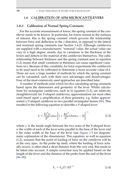
- Page 16 and 17: 6 1. BAsIC PRINCIPLEs OF ATOMIC FOR
- Page 18 and 19: 8 1. BAsIC PRINCIPLEs OF ATOMIC FOR
- Page 20 and 21: 0 1. BAsIC PRINCIPLEs OF ATOMIC FOR
- Page 22 and 23: 2 1. BAsIC PRINCIPLEs OF ATOMIC FOR
- Page 24 and 25: 4 1. BAsIC PRINCIPLEs OF ATOMIC FOR
- Page 28 and 29: 8 1. BAsIC PRINCIPLEs OF ATOMIC FOR
- Page 30 and 31: 20 1. BAsIC PRINCIPLEs OF ATOMIC FO
- Page 32 and 33: 22 1. BAsIC PRINCIPLEs OF ATOMIC FO
- Page 34 and 35: 24 1. BAsIC PRINCIPLEs OF ATOMIC FO
- Page 36 and 37: 26 1. BAsIC PRINCIPLEs OF ATOMIC FO
- Page 38 and 39: 28 1. BAsIC PRINCIPLEs OF ATOMIC FO
- Page 40 and 41: 30 1. BAsIC PRINCIPLEs OF ATOMIC FO
- Page 42 and 43: 32 2. MEASUREMENT OF PARTICLE ANd S
- Page 44 and 45: 34 2. MEASUREMENT OF PARTICLE ANd S
- Page 46 and 47: 36 2. MEASUREMENT OF PARTICLE ANd S
- Page 48 and 49: 38 2. MEASUREMENT OF PARTICLE ANd S
- Page 50 and 51: 40 2. MEASUREMENT OF PARTICLE ANd S
- Page 52 and 53: 42 2. MEASUREMENT OF PARTICLE ANd S
- Page 54 and 55: 44 2. MEASUREMENT OF PARTICLE ANd S
- Page 56 and 57: 46 2. MEASUREMENT OF PARTICLE ANd S
- Page 58 and 59: 48 2. MEASUREMENT OF PARTICLE ANd S
- Page 60 and 61: 50 2. MEASUREMENT OF PARTICLE ANd S
- Page 62 and 63: 52 2. MEASUREMENT OF PARTICLE ANd S
- Page 64 and 65: 54 2. MEASUREMENT OF PARTICLE ANd S
- Page 66 and 67: 56 2. MEASUREMENT OF PARTICLE ANd S
- Page 68 and 69: 58 2. MEASUREMENT OF PARTICLE ANd S
- Page 70 and 71: 60 2. MEASUREMENT OF PARTICLE ANd S
- Page 72 and 73: 62 2. MEASUREMENT OF PARTICLE ANd S
- Page 74 and 75: 64 2. MEASUREMENT OF PARTICLE ANd S
- Page 76 and 77:
66 2. MEASUREMENT OF PARTICLE ANd S
- Page 78 and 79:
68 2. MEASUREMENT OF PARTICLE ANd S
- Page 80 and 81:
70 2. MEASUREMENT OF PARTICLE ANd S
- Page 82 and 83:
72 2. MEASUREMENT OF PARTICLE ANd S
- Page 84 and 85:
74 2. MEASUREMENT OF PARTICLE ANd S
- Page 86 and 87:
76 2. MEASUREMENT OF PARTICLE ANd S
- Page 88 and 89:
78 2. MEASUREMENT OF PARTICLE ANd S
- Page 90 and 91:
80 2. MEASUREMENT OF PARTICLE ANd S
- Page 92 and 93:
82 3. QUANTIFICATION OF PARTICLE-BU
- Page 94 and 95:
84 3. QUANTIFICATION OF PARTICLE-BU
- Page 96 and 97:
86 3. QUANTIFICATION OF PARTICLE-BU
- Page 98 and 99:
88 3. QUANTIFICATION OF PARTICLE-BU
- Page 100 and 101:
90 3. QUANTIFICATION OF PARTICLE-BU
- Page 102 and 103:
92 3. QUANTIFICATION OF PARTICLE-BU
- Page 104 and 105:
94 3. QUANTIFICATION OF PARTICLE-BU
- Page 106 and 107:
96 3. QUANTIFICATION OF PARTICLE-BU
- Page 108 and 109:
98 3. QUANTIFICATION OF PARTICLE-BU
- Page 110 and 111:
100 3. QUANTIFICATION OF PARTICLE-B
- Page 112 and 113:
102 3. QUANTIFICATION OF PARTICLE-B
- Page 114 and 115:
104 3. QUANTIFICATION OF PARTICLE-B
- Page 116 and 117:
C H A P T E R 4 Investigating Membr
- Page 118 and 119:
4.2 THE RANgE OF POssIbILITIEs FOR
- Page 120 and 121:
4.2 THE RANgE OF POssIbILITIEs FOR
- Page 122 and 123:
4.3 CORREsPONdENCE bETwEEN sURFACE
- Page 124 and 125:
4.3 CORREsPONdENCE bETwEEN sURFACE
- Page 126 and 127:
4.4 IMAgINg IN LIqUId ANd THE dETER
- Page 128 and 129:
4.4 IMAgINg IN LIqUId ANd THE dETER
- Page 130 and 131:
4.5 EFFECTs OF sURFACE ROUgHNEss ON
- Page 132 and 133:
4.6 ‘vIsUALIsATION’ OF THE REjE
- Page 134 and 135:
4.7 THE UsE OF AFM IN MEMbRANE dEvE
- Page 136 and 137:
Dfractional 0.18 0.16 0.14 0.12 0.1
- Page 138 and 139:
4.8 CHARACTERIsATION OF METAL sURFA
- Page 140 and 141:
4.8 CHARACTERIsATION OF METAL sURFA
- Page 142 and 143:
4.8 CHARACTERIsATION OF METAL sURFA
- Page 144 and 145:
At pH 5.5, dissolution began to occ
- Page 146 and 147:
REFERENCEs 137 [4] W.R. Bowen, N. H
- Page 148 and 149:
C H A P T E R 5 AFM and Development
- Page 150 and 151:
5.2 MEAsUREMENT OF ADHEsION OF COLL
- Page 152 and 153:
5.2 MEAsUREMENT OF ADHEsION OF COLL
- Page 154 and 155:
The antibacterial activity of initi
- Page 156 and 157:
5.3 MODIFICATION OF MEMBRANEs 147 t
- Page 158 and 159:
5.3 MODIFICATION OF MEMBRANEs 149 B
- Page 160 and 161:
Force (nN m -1 ) Loading force (mN
- Page 162 and 163:
5.3 MODIFICATION OF MEMBRANEs 153 p
- Page 164 and 165:
Adhesion force (mN m -1 ) 10 8 6 4
- Page 166 and 167:
Adhesion force (mN m -1 ) 20 15 10
- Page 168 and 169:
Adhesion force (mN m -1 ) 10 8 6 4
- Page 170 and 171:
5.3 MODIFICATION OF MEMBRANEs 161 F
- Page 172 and 173:
5.4 MODIFICATION OF MEMBRANEs wITH
- Page 174 and 175:
5.4 MODIFICATION OF MEMBRANEs wITH
- Page 176 and 177:
Å 200 100 0 5.4 MODIFICATION OF ME
- Page 178 and 179:
AbbrEvIAtIonS And SyMbolS NOM Natur
- Page 180 and 181:
REFERENCEs 171 [29] W.R. Bowen, T.A
- Page 182 and 183:
174 6. NANOSCALE ANALySIS Of PHARMA
- Page 184 and 185:
176 6. NANOSCALE ANALySIS Of PHARMA
- Page 186 and 187:
178 6. NANOSCALE ANALySIS Of PHARMA
- Page 188 and 189:
180 6. NANOSCALE ANALySIS Of PHARMA
- Page 190 and 191:
182 6. NANOSCALE ANALySIS Of PHARMA
- Page 192 and 193:
184 6. NANOSCALE ANALySIS Of PHARMA
- Page 194 and 195:
186 6. NANOSCALE ANALySIS Of PHARMA
- Page 196 and 197:
188 6. NANOSCALE ANALySIS Of PHARMA
- Page 198 and 199:
190 6. NANOSCALE ANALySIS Of PHARMA
- Page 200 and 201:
192 6. NANOSCALE ANALySIS Of PHARMA
- Page 202 and 203:
194 6. NANOSCALE ANALySIS Of PHARMA
- Page 204 and 205:
196 7. MICRO/NANOENgINEERINg ANd AF
- Page 206 and 207:
198 7. MICRO/NANOENgINEERINg ANd AF
- Page 208 and 209:
200 7. MICRO/NANOENgINEERINg ANd AF
- Page 210 and 211:
202 7. MICRO/NANOENgINEERINg ANd AF
- Page 212 and 213:
204 7. MICRO/NANOENgINEERINg ANd AF
- Page 214 and 215:
206 7. MICRO/NANOENgINEERINg ANd AF
- Page 216 and 217:
208 7. MICRO/NANOENgINEERINg ANd AF
- Page 218 and 219:
210 7. MICRO/NANOENgINEERINg ANd AF
- Page 220 and 221:
212 7. MICRO/NANOENgINEERINg ANd AF
- Page 222 and 223:
214 7. MICRO/NANOENgINEERINg ANd AF
- Page 224 and 225:
216 7. MICRO/NANOENgINEERINg ANd AF
- Page 226 and 227:
218 7. MICRO/NANOENgINEERINg ANd AF
- Page 228 and 229:
220 7. MICRO/NANOENgINEERINg ANd AF
- Page 230 and 231:
222 7. MICRO/NANOENgINEERINg ANd AF
- Page 232 and 233:
224 7. MICRO/NANOENgINEERINg ANd AF
- Page 234 and 235:
226 8. ATOMIC FORCE MICROSCOPy ANd
- Page 236 and 237:
228 8. ATOMIC FORCE MICROSCOPy ANd
- Page 238 and 239:
230 8. ATOMIC FORCE MICROSCOPy ANd
- Page 240 and 241:
232 8. ATOMIC FORCE MICROSCOPy ANd
- Page 242 and 243:
234 8. ATOMIC FORCE MICROSCOPy ANd
- Page 244 and 245:
236 8. ATOMIC FORCE MICROSCOPy ANd
- Page 246 and 247:
238 8. ATOMIC FORCE MICROSCOPy ANd
- Page 248 and 249:
240 8. ATOMIC FORCE MICROSCOPy ANd
- Page 250 and 251:
242 8. ATOMIC FORCE MICROSCOPy ANd
- Page 252 and 253:
244 8. ATOMIC FORCE MICROSCOPy ANd
- Page 254 and 255:
246 9. APPLICATION OF ATOMIC FORCE
- Page 256 and 257:
248 9. APPLICATION OF ATOMIC FORCE
- Page 258 and 259:
250 9. APPLICATION OF ATOMIC FORCE
- Page 260 and 261:
252 9. APPLICATION OF ATOMIC FORCE
- Page 262 and 263:
254 9. APPLICATION OF ATOMIC FORCE
- Page 264 and 265:
256 9. APPLICATION OF ATOMIC FORCE
- Page 266 and 267:
258 9. APPLICATION OF ATOMIC FORCE
- Page 268 and 269:
260 9. APPLICATION OF ATOMIC FORCE
- Page 270 and 271:
262 9. APPLICATION OF ATOMIC FORCE
- Page 272 and 273:
264 9. APPLICATION OF ATOMIC FORCE
- Page 274 and 275:
266 9. APPLICATION OF ATOMIC FORCE
- Page 276 and 277:
268 9. APPLICATION OF ATOMIC FORCE
- Page 278 and 279:
270 9. APPLICATION OF ATOMIC FORCE
- Page 280 and 281:
272 9. APPLICATION OF ATOMIC FORCE
- Page 282 and 283:
274 9. APPLICATION OF ATOMIC FORCE
- Page 284 and 285:
276 10. FuTuRE PRosPECTs most AFM s
- Page 286 and 287:
278 10. FuTuRE PRosPECTs targeted d
- Page 288 and 289:
A Actin stress fiber, 197 Adhesion,
- Page 290:
Natural organic matter, 140 Negativ