Multivariate Taylor-Approximation - imng
Multivariate Taylor-Approximation - imng
Multivariate Taylor-Approximation - imng

Erfolgreiche ePaper selbst erstellen
Machen Sie aus Ihren PDF Publikationen ein blätterbares Flipbook mit unserer einzigartigen Google optimierten e-Paper Software.
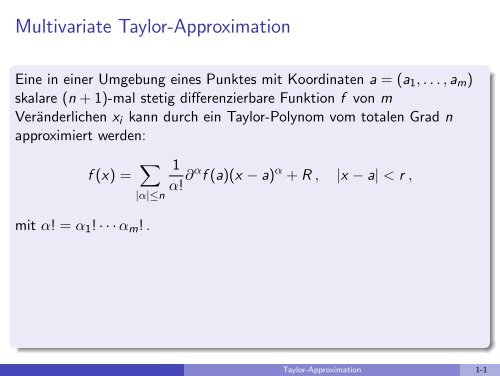
<strong>Multivariate</strong> <strong>Taylor</strong>-<strong>Approximation</strong><br />
Eine in einer Umgebung eines Punktes mit Koordinaten a = (a 1 , . . . , a m )<br />
skalare (n + 1)-mal stetig differenzierbare Funktion f von m<br />
Veränderlichen x i kann durch ein <strong>Taylor</strong>-Polynom vom totalen Grad n<br />
approximiert werden:<br />
f (x) = ∑<br />
|α|≤n<br />
mit α! = α 1 ! · · · α m ! .<br />
1<br />
α! ∂α f (a)(x − a) α + R , |x − a| < r ,<br />
<strong>Taylor</strong>-<strong>Approximation</strong> 1-1
<strong>Multivariate</strong> <strong>Taylor</strong>-<strong>Approximation</strong><br />
Eine in einer Umgebung eines Punktes mit Koordinaten a = (a 1 , . . . , a m )<br />
skalare (n + 1)-mal stetig differenzierbare Funktion f von m<br />
Veränderlichen x i kann durch ein <strong>Taylor</strong>-Polynom vom totalen Grad n<br />
approximiert werden:<br />
f (x) = ∑<br />
|α|≤n<br />
mit α! = α 1 ! · · · α m ! .<br />
Das Restglied hat die Form<br />
R =<br />
für ein θ ∈ [0, 1] .<br />
∑<br />
|α|=n+1<br />
1<br />
α! ∂α f (a)(x − a) α + R , |x − a| < r ,<br />
1<br />
α! ∂α f (u)(x − a) α , u = a + θ(x − a) ,<br />
<strong>Taylor</strong>-<strong>Approximation</strong> 1-2
Beweis:<br />
Zurückführung auf den univariaten Fall (o.B.d.A. a = 0):<br />
<strong>Taylor</strong>-<strong>Approximation</strong> 2-1
Beweis:<br />
Zurückführung auf den univariaten Fall (o.B.d.A. a = 0):<br />
setze<br />
f (x 1 , ..., x m ) = f (tx 1 , ..., tx m )| t=1 = g(t)| t=1<br />
<strong>Taylor</strong>-<strong>Approximation</strong> 2-2
Beweis:<br />
Zurückführung auf den univariaten Fall (o.B.d.A. a = 0):<br />
setze<br />
f (x 1 , ..., x m ) = f (tx 1 , ..., tx m )| t=1 = g(t)| t=1<br />
<strong>Taylor</strong>-Entwicklung der univariaten Funktion g(t) im Nullpunkt<br />
g(t) = g(0) + g ′ (0) t + · · · + 1 n! g (n) (0)t n + R<br />
mit<br />
R =<br />
1<br />
(n + 1)! g (n+1) (θt)t n+1 , θ ∈ [0, 1]<br />
<strong>Taylor</strong>-<strong>Approximation</strong> 2-3
Kettenregel ⇒<br />
g(0) =<br />
∑<br />
f (0)<br />
g ′ (0) = (∂ j f (0))x j<br />
g ′′ (0) = ∑ i<br />
.<br />
j<br />
∑<br />
(∂ i ∂ j f (0))x i x j<br />
j<br />
<strong>Taylor</strong>-<strong>Approximation</strong> 2-4
Kettenregel ⇒<br />
g(0) =<br />
∑<br />
f (0)<br />
g ′ (0) = (∂ j f (0))x j<br />
g ′′ (0) = ∑ i<br />
.<br />
j<br />
∑<br />
(∂ i ∂ j f (0))x i x j<br />
j<br />
m k Terme bei k-ter Ableitung<br />
<strong>Taylor</strong>-<strong>Approximation</strong> 2-5
Kettenregel ⇒<br />
g(0) =<br />
∑<br />
f (0)<br />
g ′ (0) = (∂ j f (0))x j<br />
g ′′ (0) = ∑ i<br />
.<br />
j<br />
∑<br />
(∂ i ∂ j f (0))x i x j<br />
j<br />
m k Terme bei k-ter Ableitung<br />
Zusammenfassen gleicher partieller Ableitungen <br />
Koeffizienten der Entwicklung<br />
z.B. für m = 2, k = 5, Zusammenfassung von<br />
∂ 1 ∂ 1 ∂ 1 ∂ 2 ∂ 2 , ∂ 1 ∂ 2 ∂ 1 ∂ 2 ∂ 1 , ∂ 1 ∂ 2 ∂ 2 ∂ 1 ∂ 1 , ...<br />
∂ α , α = (3, 2) ( )<br />
5<br />
3 = 5!/(3! 2!) Terme<br />
<strong>Taylor</strong>-<strong>Approximation</strong> 2-6
allgemein<br />
( ) ( ) ( )<br />
k k − α1 k − α1 − . . . − α m−1<br />
· · · ·<br />
= k!/(α 1 ! . . . α m !)<br />
α 1 α 2 α m<br />
Terme, wenn nach der ν-ten Komponente jeweils α ν -mal abgeleitet wird<br />
Einsetzen der Ableitungen der Funktion g(t) , Kürzen des Faktors k! <br />
Entwicklung von f<br />
<strong>Taylor</strong>-<strong>Approximation</strong> 2-7
Beispiel:<br />
<strong>Taylor</strong>-Entwicklung einer Funktion von zwei Variablen:<br />
f (x, y) = f + f x (x − x 0 ) + f y (y − y 0 )<br />
+ f xx<br />
2 (x − x 0) 2 + f xy (x − x 0 ) (y − y 0 ) + f yy<br />
2 (y − y 0) 2<br />
+ f xxx<br />
6 (x − x 0) 3 + f xxy<br />
2 (x − x 0) 2 (y − y 0 )<br />
+ f xyy<br />
2 (x − x 0) (y − y 0 ) 2 + f yyy<br />
6 (y − y 0) 3 + R ,<br />
wobei f und sämtliche partielle Ableitungen im Punkt (x 0 , y 0 ) ausgewertet<br />
werden<br />
<strong>Taylor</strong>-<strong>Approximation</strong> 3-1
Beispiel:<br />
<strong>Taylor</strong>-Entwicklung einer Funktion von zwei Variablen:<br />
f (x, y) = f + f x (x − x 0 ) + f y (y − y 0 )<br />
+ f xx<br />
2 (x − x 0) 2 + f xy (x − x 0 ) (y − y 0 ) + f yy<br />
2 (y − y 0) 2<br />
+ f xxx<br />
6 (x − x 0) 3 + f xxy<br />
2 (x − x 0) 2 (y − y 0 )<br />
+ f xyy<br />
2 (x − x 0) (y − y 0 ) 2 + f yyy<br />
6 (y − y 0) 3 + R ,<br />
wobei f und sämtliche partielle Ableitungen im Punkt (x 0 , y 0 ) ausgewertet<br />
werden<br />
Entwickeln von<br />
im Punkt (x 0 , y 0 ) = (0, 0)<br />
f (x, y) = sin(x − ωy)<br />
<strong>Taylor</strong>-<strong>Approximation</strong> 3-2
wegen<br />
∂ α x ∂ β y f (0, 0) = sin (α+β) (0) (−ω) β<br />
<strong>Approximation</strong><br />
sin(x − ωy) = x − ωy − 1 6 (x 3 − 3ωx 2 y + 3ω 2 xy 2 − ω 3 y 3 ) +R<br />
} {{ }<br />
(x−ωy) 3<br />
<strong>Taylor</strong>-<strong>Approximation</strong> 3-3
wegen<br />
∂ α x ∂ β y f (0, 0) = sin (α+β) (0) (−ω) β<br />
<strong>Approximation</strong><br />
mit<br />
sin(x − ωy) = x − ωy − 1 6 (x 3 − 3ωx 2 y + 3ω 2 xy 2 − ω 3 y 3 ) +R<br />
} {{ }<br />
(x−ωy) 3<br />
für ein θ ∈ [0, 1]<br />
R = 1 4! (f x 4 + 4f x 3 y + 6f x 2 y 2 + 4f xy 3 + f y 4)(θ(x, y))<br />
= 1 4! (x − ωy)4 sin(θ(x − ωy))<br />
<strong>Taylor</strong>-<strong>Approximation</strong> 3-4
Alternative Berechnung des <strong>Taylor</strong>-Polynoms: durch Einsetzen von<br />
t = x − ωy in die eindimensionale Reihendarstellung der Sinusfunktion:<br />
t = x − ωy <br />
sin(t) = t − t3<br />
3! + t5<br />
5! − ... .<br />
<strong>Taylor</strong>-<strong>Approximation</strong> 3-5
Alternative Berechnung des <strong>Taylor</strong>-Polynoms: durch Einsetzen von<br />
t = x − ωy in die eindimensionale Reihendarstellung der Sinusfunktion:<br />
t = x − ωy <br />
sin(t) = t − t3<br />
3! + t5<br />
5! − ... .<br />
f (x, y) = (x − ωy) − 1 3! (x − ωy)3 + 1 cos(θ)(x − ωy)5<br />
5!<br />
(univariates Restglied)<br />
<strong>Taylor</strong>-<strong>Approximation</strong> 3-6
Beispiel:<br />
Entwicklung des Polynoms<br />
f (x, y, z) = z 2 − xy<br />
an der Stelle (0, −2, 1)<br />
<strong>Taylor</strong>-<strong>Approximation</strong> 4-1
Beispiel:<br />
Entwicklung des Polynoms<br />
f (x, y, z) = z 2 − xy<br />
an der Stelle (0, −2, 1)<br />
von Null verschiedene Ableitungen<br />
f x = −y , f y = −x , f z = 2z , f xy = −1 , f zz = 2<br />
Auswerten am Entwicklungspunkt <strong>Taylor</strong>-Darstellung<br />
1 + 2x + (−0)(y + 2) + 2(z − 1) + (−1)x(y + 2) + 1 2 2(z − 1)2 = z 2 − xy<br />
<strong>Taylor</strong>-<strong>Approximation</strong> 4-2
Beispiel:<br />
Entwicklung des Polynoms<br />
f (x, y, z) = z 2 − xy<br />
an der Stelle (0, −2, 1)<br />
von Null verschiedene Ableitungen<br />
f x = −y , f y = −x , f z = 2z , f xy = −1 , f zz = 2<br />
Auswerten am Entwicklungspunkt <strong>Taylor</strong>-Darstellung<br />
1 + 2x + (−0)(y + 2) + 2(z − 1) + (−1)x(y + 2) + 1 2 2(z − 1)2 = z 2 − xy<br />
alternativ: Entwicklung durch Umformung<br />
<strong>Taylor</strong>-<strong>Approximation</strong> 4-3
Beispiel:<br />
Entwicklung des Polynoms<br />
f (x, y, z) = z 2 − xy<br />
an der Stelle (0, −2, 1)<br />
von Null verschiedene Ableitungen<br />
f x = −y , f y = −x , f z = 2z , f xy = −1 , f zz = 2<br />
Auswerten am Entwicklungspunkt <strong>Taylor</strong>-Darstellung<br />
1 + 2x + (−0)(y + 2) + 2(z − 1) + (−1)x(y + 2) + 1 2 2(z − 1)2 = z 2 − xy<br />
alternativ: Entwicklung durch Umformung<br />
substituiere<br />
y + 2 = η , z − 1 = ζ<br />
<br />
f (x, y, z) = (ζ + 1) 2 − x(η − 2) = ζ 2 + 2ζ + 1 − xη + 2x<br />
<strong>Taylor</strong>-<strong>Approximation</strong> 4-4