Phys. Dirk Burghardt

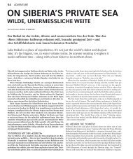
93
Anhang B
Herleitung des Abstandes a i in Formel (3.2-4)
Ausgangspunkt der Herleitung ist die Abstandsberechnung für die Punkte P 0 bzw. P i .
P
j +1
d i , j+1
a 2 i = (x 0 − x i ) 2 + (y 0 − y i ) 2
P 0 wandert entlang der Strecke P j P j+1
:
(B.1)
P
d j , j+1
P
0
j
a
i
d i , j
Einsetzen von (B.2) in (B.1) führt zu
P
i
x 0 = x j + ∆x · t , y 0 = y j + ∆y · t , (B.2)
wobei gilt
∆x = x j+1 − x j , ∆y = y j+1 − y j . (B.3)
a 2 i = (x j − x i + ∆x · t) 2 + (y j − y i + ∆y · t) 2 (B.4)
= (x j − x i ) 2 + (∆x · t) 2 + 2(x j − x i )(∆x · t) + (B.5)
(y j − y i ) 2 + (∆y · t) 2 + 2(y j − y i )(∆y · t) (B.6)
= d 2 ij + d 2 jj+1t 2 + 2t [(x j − x i )∆x + (y j − y i )∆y] . (B.7)
Mit der Randbedingung für t = 1 und a i = d ij+1 in Formel (B.7) folgt
d 2 ij+1 = d 2 ij + d 2 jj+1 + 2 [(x j − x i )∆x + (y j − y i )∆y] . (B.8)
Ersetzen der eckigen Klammer durch Substitution von (B.8) in (B.7) führt zur gesuchten Gleichung.