Gradientenbasierte Rauschfunktionen und Perlin Noise - Campus ...
Gradientenbasierte Rauschfunktionen und Perlin Noise - Campus ...
Gradientenbasierte Rauschfunktionen und Perlin Noise - Campus ...

Sie wollen auch ein ePaper? Erhöhen Sie die Reichweite Ihrer Titel.
YUMPU macht aus Druck-PDFs automatisch weboptimierte ePaper, die Google liebt.
Burger: <strong>Gradientenbasierte</strong> <strong>Rauschfunktionen</strong> <strong>und</strong> <strong>Perlin</strong> <strong>Noise</strong> 26<br />
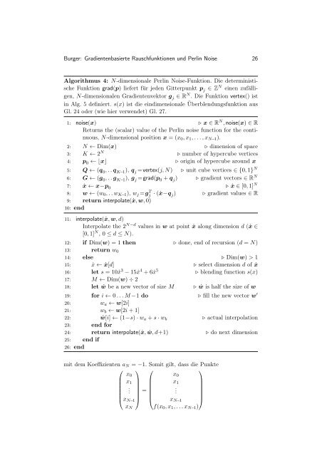
Algorithmus 4: N-dimensionale <strong>Perlin</strong> <strong>Noise</strong>-Funktion. Die deterministische<br />
Funktion grad(p) liefert für jeden Gitterpunkt p j ∈ Z N einen zufälligen,<br />
N-dimensionalen Gradientenvektor g j ∈ R N . Die Funktion vertex() ist<br />
in Alg. 5 definiert. s(x) ist die eindimensionale Überblendungsfunktion aus<br />
Gl. 24 oder (wie hier verwendet) Gl. 27.<br />
1: noise(x) ⊲ x ∈ R N , noise(x) ∈ R<br />
Returns the (scalar) value of the <strong>Perlin</strong> noise function for the continuous,<br />
N-dimensional position x = (x0,x1,...,xN−1).<br />
2: N ← Dim(x) ⊲ dimension of space<br />
3: K ← 2 N ⊲ number of hypercube vertices<br />
4: p 0 ← ⌊x⌋ ⊲ origin of hypercube aro<strong>und</strong> x<br />
5: Q ← (q 0,..q K−1), q j=vertex(j,N) ⊲ unit cube vertices ∈ {0,1} N<br />
6: G ← (g 0,..g K−1), g j=grad(p 0 +q j) ⊲ gradient vectors ∈ R N<br />
7: ˙x ← x−p 0 ⊲ ˙x ∈ [0,1] N<br />
8: w ← (w0,..wK−1), wj=g T j ·(˙x−q j) ⊲ gradient values ∈ R<br />
9: return interpolate(˙x,w,0)<br />
10: end<br />
11: interpolate(˙x,w,d)<br />
Interpolate the 2 N−d values in w at point ˙x along dimension d (˙x ∈<br />
[0,1] N , 0 ≤ d ≤ N).<br />
12: if Dim(w) = 1 then ⊲ done, end of recursion (d = N)<br />
13: return w0<br />
14: else ⊲ Dim(w) > 1<br />
15: ˙x ← ˙x[d] ⊲ select dimension d of ˙x<br />
16: let s = 10˙x 3 −15˙x 4 +6˙x 5 ⊲ blending function s(x)<br />
17: M ← Dim(w)÷2<br />
18: let ´w be a new vector of size M ⊲ ´w is half the size of w<br />
19: for i ← 0...M−1 do ⊲ fill the new vector w ′<br />
20: wa ← w[2i]<br />
21: wb ← w[2i+1]<br />
22: ´w[i] ← (1−s)·wa +s·wb ⊲ actual interpolation<br />
23: end for<br />
24: return interpolate(˙x, ´w,d+1) ⊲ do next dimension<br />
25: end if<br />
26: end<br />
mit dem Koeffizienten aN = −1. Somit gilt, dass die Punkte<br />
⎛ ⎞ ⎛ ⎞<br />
⎜<br />
⎝<br />
x0<br />
x1<br />
.<br />
xN−1<br />
xN<br />
⎟ ⎜<br />
⎟ ⎜<br />
⎟ ⎜<br />
⎟ = ⎜<br />
⎟ ⎜<br />
⎠ ⎝<br />
x0<br />
x1<br />
.<br />
xN−1<br />
f(x0,x1,...xN−1)<br />
⎟<br />
⎠