Über hyperbolische Funktionen 2 ee xsinh − = 2 ee x cosh + = sinh x ...

Über hyperbolische Funktionen
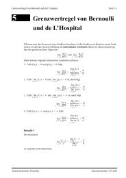
Für eine Reihe von Anwendungen insbesondere in der Physik erweist es sich als vorteilhaft,
Funktionen zu definieren, die sich aus einfachen Exponentialfunktionen zusammensetzen.
Die Funktionen „sinus hyperbolikus“ bzw. „cosinus hyperbolikus“ sind
wie folgt definiert:
x −x
x −x
e − e
e + e
sinh x =
cosh x =
2
2
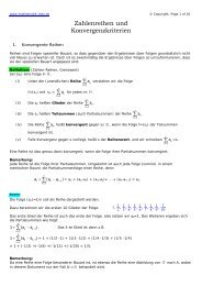
Wie in der Grafik zu sehen, ist
cosh x eine gerade Funktion, da cosh x = cosh (-x)
sinhx dagegen eine ungerade, da
sinh x = -sinh (-x).
Interessant ist cosh x. Für diese Funktion gilt cosh x ≥ 1 .
In der Technik stellt sie die Gleichgewichtslinie einer in zwei
Punkten aufgehängten Kette (Kettenlinie) oder auch einen
freistehenden Bogen dar (Gateway Arch; St. Louis, Missouri;
USA).
Interessant ist das Verhalten der beiden Funktionen für x → ∞ . Da die Funktion e -x für große x
gegen 0 geht, streben letztendlich sowohl sinh x, als auch cosh x gegen e x /2.
Wie leicht zu sehen ergibt sich außerdem (einfach ausrechnen):
e cosh x sinh x
x
= + ; e cosh x sinh x
x −
= − ;
2
2
cosh x − sinh x = 1
Weiterhin ergeben sich folgende Zusammenhänge:
e
2⋅
cosh x ⋅sinh
x =
cosh 2x
+
sinh 2x
2x
e
=
− e
2
2x
−2x
+ e
2
und allgemeiner die Additionstheoreme:
=
−2x
sinh 2x
=
cos2x
sinh x ⋅ cosh y ± cosh x ⋅sinh
y = sinh( x ±
cosh x ⋅ cosh y ± sinh x ⋅sinh
y = cosh( x ±
Die gezeigten Zusammenhänge haben eine auffällige Ähnlichkeit mit den (hoffentlich!) bekannten
Beziehungen der trigonometrischen Funktionen. Den Grund dafür gibt’s später!
Dr. Hempel – Mathematische Grundlagen , Hyperbolische Funktionen Seite 1
y)
y)

Desweiteren gilt:
2tanh
x
tanh 2x
2
1+
tanh x
= ;
Die Funktionen „Tangens Hyperbolikus“ und Kotangens Hyperbolikus“
werden folgendermaßen definiert:
sinh x e −e
tanh x
−
cosh x e + e
cosh x
sinh x
x −x
x −x
= = x coth x =
x
= x −x
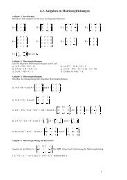
Daraus ergibt sich: tanh x < 1 und coth x > 1.
tanh x ist über den gesamten Definitionsbereich stetig.
coth x ist unstetig bei x = 0.
Beide Funktionen haben einen Grenzwert von
1 für x → ∞ und von -1 für x → -∞ .
tanh( x
Ableitungen von: cosh x, sinh x, tanh x, coth x
±
y)
tanh x ± tanh y
=
1±
tanh x ⋅tanh
y
Betrachtet man die hyperbolischen Funktionen in ihrer Darstellung mittels e-Funktion, ist leicht zu
erkennen daß:
• (cosh x)
′ = sinh x
• (sinh x)
′ = cosh x
′
2
2
sinh x cosh x −sinh
x 1
2
• (tanh x)
′ =
⎛ ⎞
⎜ ⎟ =
= = 1−
tanh x
2
2
⎝ cosh x ⎠ cosh x cosh x
′
2
2
cosh x sinh x − cosh x 1
2
• (coth x)
′ =
⎛ ⎞
⎜ ⎟ =
= − = 1−
coth x
2
2
⎝ sinh x ⎠ sinh x sinh x
Areafunktion als Umkehrfunktion der hyperbolischen Funktion
Die Bezeichnung Areafunktion entspringt dem Zusammenhang dieser Funktion mit dem Flächeninhalt
(area) eines Hyperbelsektors.
Wie bekannt, entsteht eine Umkehrfunktion durch das Vertauschen der unabhängigen und der abhän-
gigen Variablen, hier also y und x.
Man könnte als z.B. schreiben: x = cosh y – oder, um die gewohnte Schreibweise (unabhängige Va-
riable getrennt auf der linken Seite) beizubehalten: y = arcosh x. Die Funktion heisst Area-Kosinus-
Hyperbolikus und ist die Umkehrfunktion zum Kosinus-Hyperbolikus. Es gilt also:
y −y
e + e
2y
y
x = oder e 2xe
+ 1=
0
2
e
y
− und damit
2
2
= x ± x −1
⇒ y =
arcosh
x = ln( x ± x −1)
Dr. Hempel – Mathematische Grundlagen , Hyperbolische Funktionen Seite 2
e
e
+ e
−e

Nach dem gleichen Muster erhält man auch Ausdrücke für die übrigen Areafunktionen, so dass sich
letztendlich ergibt:
ar cosh x
=
arsinh
x = ln( x +
2
x
ar tanh x = ln
1+
x
1−
x
ar coth x = ln
x + 1
x −1
Die Ableitungen der Areafunktionen ergeben sich zu:
1
( arcoshx)
′ =
2
± x
1
( artanhx)
′ = 2
1−
x
Es ist zu beachten, dass der Logarithmus definitionsgemäß
kein negatives Argument haben darf!
−1
1
( arsinhx)
′ =
2
+ x
1
( arcothx)
′ = 2
1−
x
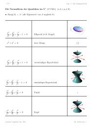
Warum hyperbolische Funktionen ? - Zusammenhang mit der Hyperbel
So wie sich viele Funktionen in der sogenannten „Parameterform“ darstellen lassen, geht das auch mit
der Hyperbel – mit Hilfe der hyperbolischen Funktionen. Mit
x = ± a cosh t und y = bsinh
t
ergibt sich durch Umstellen und eliminieren des Parameters t:
2 2
x 2
2
= cosh t − sinh
2 2
a
ln( x
y
−
b
±
x
2
−1)
+ 1)
t = 1
Beachtet man das doppelte Vorzeichen, ergibt sich der bekannte analytische Ausdruck für
eine Hyperbel.
Dr. Hempel – Mathematische Grundlagen , Hyperbolische Funktionen Seite 3
+ 1