Nicola Arndt und Matthias Pohl - Neobiota

Anwendung und Auswertung der
Karte der natürlichen Vegetation Europas
Application and Analysis of the
Map of the Natural Vegetation of Europe
BfN-Skripten 156
2005

Anwendung und Auswertung der
Karte der natürlichen Vegetation Europas
Application and Analysis of the
Map of the Natural Vegetation of Europe
Beiträge und Ergebnisse des internationalen
Workshops auf der Insel Vilm, Deutschland,
7. bis 11. Mai 2001
Proceedings of the International Workshop, held on the
Island of Vilm, Germany, 7-11 May 2001
zusammengestellt und bearbeitet von/
compiled and revised by
Udo Bohn
Christoph Hettwer
Gisela Gollub

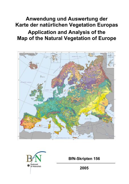
Titelbild / Cover: Verkleinerung der Übersichtskarte der natürlichen Vegetation Europas 1 : 10 Mio.
Reduced General Map of the Natural Vegetation of Europe 1 : 10 million
Bearbeitung / Compilation: Dr. Udo Bohn, Christoph Hettwer, Gisela Gollub
Bundesamt für Naturschutz, Bonn/
Federal Agency for Nature Conservation, Bonn, Germany
Zitiervorschlag / Proposal for citation:
BOHN, U.; HETTWER, C. & GOLLUB, G. [Bearb./Eds.] (2005): Anwendung und Auswertung der Karte der
natürlichen Vegetation Europas / Application and Analysis of the Map of the Natural Vegetation of Europe. –
Bonn (Bundesamt für Naturschutz) – BfN-Skripten 156: 452 S./p.
Diese Veröffentlichung wird aufgenommen in die Literaturdatenbank DNL-online (www.dnl-online.de).
This publication is included in the literature database DNL-online (www.dnl-online.de).
Herausgeber/Publisher: Bundesamt für Naturschutz (BfN)/Federal Agency for Nature Conservation
Konstantinstr. 110, 53179 Bonn, Germany
Tel: (+49) 228/8491-0, Fax: (+49) 228/8491-9999
URL: http://www.bfn.de
Das Werk ist einschließlich aller seiner Teile urheberrechtlich geschützt. Jede Verwertung außerhalb der engen
Grenzen des Urheberrechtsgesetzes ist ohne Zustimmung des Herausgebers unzulässig und strafbar. Dies gilt
insbesondere für Vervielfältigungen, Übersetzungen, Mikroverfilmungen und die Einspeicherung und
Verarbeitung in elektronischen Systemen.
Nachdruck, auch in Auszügen, und Vervielfältigung nur mit Genehmigung des BfN.
This work with all its parts is protected by copyright. Any use beyond the strict limits of the copyright law without
the consent of the Bundesamt für Naturschutz is inadmissible and punishable. No part of the material protected
by this copyright notice may be reproduced or utilized in any form or by any means, electronic or mechanical,
including photocopying, recording or by any information storage and retrieval system without written permission
from the copyright owner.
Reprints, even excerpt reprints, and reproduction permitted only with consent of the BfN.
Der Herausgeber übernimmt keine Gewähr für die Richtigkeit, die Genauigkeit und Vollständigkeit der
Angaben sowie für die Beachtung privater Rechte Dritter. Die in den Beiträgen geäußerten Ansichten und
Meinungen müssen nicht mit denen des Herausgebers übereinstimmen.
The publisher takes no guarantee for correctness, details and completeness of statements and views in this
report as well as no guarantee for respecting private rights of third parties.
Views expressed in the papers published in this issue of BfN-Skripten are those of the authors and do not
necessarily represent those of the publisher.
Druck/Print: BMU-Druckerei
Gedruckt auf 100% Altpapier/Printed on 100% recycled paper
Bonn, Germany 2005

Inhalt / Contents
Vorwort / Resolution der Teilnehmer des Workshops..................................................................................7
Foreword / Resolution of the Participants of the Workshop .......................................................................11
UDO BOHN
Einführung in den Internationalen Workshop über Anwendung und Auswertung der Karte der
natürlichen Vegetation Europas / ................................................................................................................15
Introduction to the International Workshop on the Application and Analysis of the Map of the
Natural Vegetation of Europe .....................................................................................................................20
Ökologische Raumgliederung / Ecological Area Cassification
MARCO PAINHO & GABRIELA AUGUSTO
A Digital Map of European Ecological Regions / Digitale Karte der Ökologischen Regionen Europas ...27
WINFRIED SCHRÖDER
Die Potentielle Natürliche Vegetation als Datengrundlage einer ökologischen Raumgliederung /
Using the Map of the Natural Vegetation for an Classification of Terrestrial Ecoregions .........................37
HENK SIMONS
Global Ecological Zoning for the FAO Global Forest Resources Assessment 2000 / Entwicklung
einer globalen ökologischen Zonierung für die weltweite Bewertung der Waldressourcen im Jahr
2000 seitens der FAO..................................................................................................................................55
JOHN MORRISON & DAVID M. OLSON
The Natural Vegetation Map of Europe: A Regional Source for WWF’s Terrestrial Ecoregions of
the World / Die Karte der natürlichen Vegetation Europas als regionale Grundlage für die WWF-
Karte der terrestrischen Ökoregionen der Welt.......................................................................................... 71
DIRK M. WASCHER
The Role of Natural Vegetation Data for European Landscape Mapping and Assessment / Die
Rolle von Daten zur natürlichen Vegetation bei der Kartierung und Bewertung europäischer Land-
schaftstypen.................................................................................................................................................81
GALINA N. OGUREEVA
Vegetation Classification for the Map “Zones and altitudinal zonality types of the vegetation of
Russia and adjacent territories” / Die Vegetationsgliederung in der Karte „Vegetationszonen und
Höhenstufen in Rußland und angrenzenden Gebieten“ ............................................................................113
ARVE ELVEBAKK
Climatic Gradients as Reflected in the Vegetation Zones of the Northernmost Part of the Map of
The Natural Vegetation of Europe / Klimagradienten, die sich in der Vegetationszonierung im
Nördlichen Teil der Karte der natürlichen Vegetation Europas widerspiegeln ........................................123
Gliederung und Inhalte einzelner Formationen / Classification and Content of Individual
Formations
VLADISLAV I. VASILEVICH
Karte der natürlichen Vegetation Europas und Klassifizierung der borealen Wälder / Map of the
Natural Vegetation of Europe and Classification of the Boreal Forest Vegetation...................................137
KAMIL RYBNÍČEK
Regional Mire Complex Types in Europe /Regionale Moorkomplex-Typen in Europa ..........................143
IRINA N. SAFRONOVA
The Ecological Classification of Desert and Steppe Vegetation on the European Vegetation Map /
Ökologische Gliederung der Wüsten- und Steppenvegetation in der Karte der natürlichen
Vegetation Europas ...................................................................................................................................151
3

Erhaltungszustand der natürlichen Vegetation und deren Repräsentanz in
Schutzgebietssystemen / Conservation Status of the Natural Vegetation and its
Representation in Protected Areas Networks
HANS D. KNAPP
Vegetationsregionen und Schutzgebiete in Europa / Vegetation Regions and Protected Areas in
Europe .......................................................................................................................................................165
DOUG EVANS
Some Uses of the Map of the Natural Vegetation of Europe for Natura 2000 / Anwendung der
Karte der natürlichen Vegetation Europas für Natura 2000 ......................................................................195
LARS PÅHLSSON
Evaluating Vegetation Types for Nature Conservation and Monitoring of Landscape Development
Applied in the Nordic Countries / Bewertung von Vegetationstypen für den Naturschutz und zur
Überwachung der Landschaftsentwicklung am Beispiel der Nordischen Länder.....................................205
ZDENKA NEUHÄUSLOVÁ
Vergleich der aktuellen Vegetation der Tschechischen Republik mit der potentiellen natürlichen
Vegetation (tschechische und Europakarte) und deren Vertretung im vorhandenen Schutzgebietssystem
/ Comparison of the Current Vegetation of the Czech Republic with the Potential Natural
Vegetation (Czech and European Maps) and its Representation in the Existing Network of
Protected Areas..........................................................................................................................................215
NICOLAE DONIŢĂ & DOINA IVAN
Auswertung der Vegetationskarte von Europa für Rumänien: Erhaltungszustand der natürlichen
Vegetation und Schutzmaßnahmen / Application of the European Vegetation Map for Romania:
Present State of the Natural Vegetation and Measures for its Protection..................................................227
FRANCO PEDROTTI
Erhaltungszustand der natürlichen Vegetation und deren Repräsentanz in Schutzgebietssystemen
in Italien / State of Conservation of the Natural Vegetation and its Representation in the Protected
Areas Network of Italy ..............................................................................................................................233
NUGZAR ZAZANASHVILI
Application of the Map of the Natural Vegetation of Europe in Developing a Protected Areas
Network in the Caucasus Ecoregion / Verwendung der Karte der natürlichen Vegetation Europas
beim Aufbau eines Schutzgebietssystems in der Kaukasus-Ökoregion ....................................................251
CHRISTOPH HETTWER
Karte der natürlichen Vegetation Europas als Grundlage für den Aufbau eines repräsentativen
Schutzgebietssystems, Beispiel NATURA 2000 für Deutschland / Map of the Natural Vegetation
of Europe as a Basis for the Establishment of a Representative System of Protected Areas: the
Example of NATURA 2000 in Germany..................................................................................................263
Untersuchungen zur Naturnähe, Bestandesstruktur und Artenvielfalt / Investigation
of Naturalness, Stand Structure and Species Diversity
HEINZ SCHLÜTER
Vergleich der potentiell-natürlichen mit der heutigen realen Vegetation zur Ableitung ihres Natürlichkeitsgrades
/ Comparison of the Potential Natural and Current Vegetation as a Means of Determining
its Degree of Naturalness ..............................................................................................................277
PETER VESTERGAARD
Natural and Current Vegetation of Denmark with Reference to Biodiversity / Natürliche und
Aktuelle Vegetation Dänemarks unter Berücksichtigung der Biodiversität ..........................................285
4

MARTIN JENSSEN & GERHARD HOFMANN
Zur Quantifizierung von Naturnähe und Phytodiversität in Waldungen auf der Grundlage der
potentiellen natürlichen Vegetation / On Quantification of Naturalness and Phytodiversity in
Forests Based on Potential Natural Vegetation.........................................................................................297
Auswertung der Europakarte für synsystematische Gliederungen / Analysis of the
European Vegetation Map for Synsystematic Classifications
PAUL HEISELMAYER
Die Kartierungseinheiten der Europakarte als Grundlage für die Verbreitung und chorologische
Typisierung von Pflanzengesellschaften am Beispiel der alpinen Vegetation / Mapping Units of
the European Vegetation Map as a Basis for Distribution and Chorological Characterization of
Plant Communities: Examples from Alpine Vegetation ...........................................................................317
GIORGI NAKHUTSRISHVILI
Gliederung der Hochgebirgsvegetation des Kaukasus (im Vergleich zu den Alpen) / Caucasian
High Mountain Vegetation (in Comparison with that of the Alps)...........................................................335
JOOP H.J. SCHAMINÉE, STEPHAN M. HENNEKENS & RENSE HAVEMAN
Towards a European Expert System for the Management of Species, Vegetation and Landscapes /
Aufbau eines europäischen Informationssystems für die Verknüpfung von Daten über
Pflanzenarten, Vegetation und Landschaften............................................................................................347
Anwendung der Europakarte bei der Wiederherstellung der natürlichen Vegetation
und von alten Kulturlandschaften / Use of the European Vegetation Map for Restoration
of Natural Vegetation and Old Cultural Landscapes
JOHN R. CROSS
The Use of the Map of the Natural Vegetation of Europe in the Conservation and Creation of Native
Woodlands in Ireland / Anwendung der Karte der natürlichen Vegetation Europas für Erhalt und
Schaffung indigener Wälder in Irland.......................................................................................................361
JOHN RODWELL
Restoring Cultural Landscapes Using the Vegetation Map of Europe / Wiederherstellung von
Kulturlandschaften mit Hilfe der Karte der Natürlichen Vegetation Europas ..........................................371
Anwendung der Europakarte für Forstwirtschaft, naturnahen Waldbau und im
Hinblick auf Auswirkungen von Klimaänderungen / Use of the European Vegetation
Map in Silviculture, Ecosystem-based Forestry, and with Respect to the Effects of
Climate Change
PETER A. SCHMIDT
Die potentielle natürliche Vegetation unter dem Aspekt der Waldentwicklung und naturnaher
Waldbewirtschaftung an ausgewählten Beispielen ost- und mitteleuropäischer Waldgebiete /
Potential Natural Vegetation with Regard to Forest Development and Ecosystem-based Forest
Management: Selected Examples from Eastern and Central European Forest Areas...............................383
HANS-PETER KAHLE, RÜDIGER UNSELT & HEINRICH SPIECKER
Forest Ecosystems in a Changing Environment: Growth Patterns as Indicators for Stability of
Norway Spruce Forests within and beyond the Limits of their Natural Range / Waldökosyteme in
einer sich verändernden Umwelt: Wachstumsmuster als Indikatoren für die Stabilität von Fichtenwäldern
innerhalb und außerhalb ihres natürlichen Verbreitungsgebiets .................................................399
GERHARD HOFMANN & MARTIN JENSSEN
Potentielle natürliche Waldvegetation und Naturraumpotentiale: Quantifizierung natürlicher
Potentiale der Nettoprimärproduktion und der Kohlenstoffspeicherung / Potential Natural Forest
Vegetation and Natural Landscape Potential: Quantification of Natural Potential of Net Primary
Production and Carbon Storage.................................................................................................................411
5

HOLGER FREUND
Holozäne Meeresspiegel-Schwankungen und Landschaftsentwicklung in der südlichen Nordsee /
Holocene Sea Level Fluctuations and Landscape Development in the Southern North Sea.....................429
GIAN-RETO WALTHER
Anwendung (und Auswertung) der Karte der natürlichen Vegetation Europas für Auswirkungen
und Szenarios von Klimaänderungen / Application (and Analysis) of the Map of the Natural
Vegetation of Europe with Regard to the Impacts and Scenarios of Climate Change ..............................439
6

Vorwort
Vom 07. bis 10. Mai 2001 fand an der Internationalen Naturschutzakademie Insel Vilm ein vom Bundes-
amt für Naturschutz durchgeführter Internationaler Workshop zur „Anwendung und Auswertung der Karte
der natürlichen Vegetation Europas“ statt.
Ziel war die Vorstellung der digitalisierten und gedruckten gesamteuropäischen Vegetationskarte im Hin-
blick auf ihre Anwendungs- und Auswertungsmöglichkeiten für Vegetationskunde, Naturschutz, Land-
schaftsökologie, Landschaftsplanung und eine naturverträgliche, nachhaltige Nutzung auf europäischer,
nationaler und regionaler Ebene.
An der Veranstaltung nahmen 44 eingeladene Experten aus 18 Ländern Europas teil, die im Kartenprojekt
mitgearbeitet haben bzw. Anwender und Nutzer der Ergebnisse repräsentieren. Es wurden insgesamt 34
Anwendungs- und Auswertungsbeispiele zu verschiedenen Oberthemen vorgestellt und diskutiert.
Zu den vielfältigen Möglichkeiten der Anwendung und Auswertung der im Bundesamt für Naturschutz
(BfN) – und nun auch auf CD-ROM – digital vorliegenden Daten der natürlichen Vegetation Europas im
Maßstab 1:2,5 Millionen gehören Überlagerungen und Verschneidungen mit anderen Landschafts- und
Ökosysteminformationen wie Flächennutzung, Waldverteilung, Bestände naturnaher Vegetation, Schutzgebiete,
Artenverbreitung, Bioproduktion, Klimadaten u. a.
Auf dem internationalen Workshop wurden schwerpunktmäßig folgende Themen behandelt: Ökologische
Raumgliederung, natürliche Biodiversität und deren anthropogene Veränderung, Erhaltungszustand und
Wiederherstellung der natürlichen Vegetation, Aufbau repräsentativer Schutzgebietssysteme (z. B. im
Rahmen von NATURA 2000), Vergleich der aktuellen und potentiellen Bioproduktivität, Anwendung in
der Landschaftsplanung, in der Forstwirtschaft und für naturnahen Waldbau sowie Auswirkung von Klimaänderungen.
Nach der Veröffentlichung des dreiteiligen Druckwerkes „Karte der Natürlichen Vegetation Europas“ mit
umfangreichem Erläuterungstext, Legendenband und Kartenteil (im Jahr 2003) sowie der Interaktiven CD-
ROM (2004), die alle Karten- und Textinformationen nun insgesamt auch digital – in deutscher und englischer
Version – zur Verfügung stellt, wird das Gesamtwerk durch diese Veröffentlichung der Tagungsbeiträge
abgerundet. Sie liefert wertvolle Anregungen und praktische Hinweise, wie das umfangreiche und
auf europäischer Ebene einzigartige Informationsmaterial zum Nutzen von Natur und Landschaft und im
Hinblick auf eine naturverträgliche und nachhaltige Nutzung der Naturgüter eingesetzt werden kann.
Prof. Dr. Hartmut Vogtmann
Präsident des Bundesamtes für Naturschutz
7

Resolution der Teilnehmer des Workshops im Mai 2001: Ergebnisse und Schlußfolgerungen
1) Die Karte der natürlichen Vegetation Europas (1:2,5 Mio. in 9 Blättern und Übersichtskarte
1:10 Mio.) ist das Ergebnis mehr als zwanzigjähriger Zusammenarbeit von in der Vegetations-
geographie, -ökologie und -kartographie führenden Wissenschaftlern und Institutionen aus 31 euro-
päischen Ländern. Da die Karte Gesamteuropa in seinen geographischen Grenzen – bis zum Ural und
einschließlich der Kaukasusländer – abdeckt, stellt sie erstmalig wichtiges ökologisches Basismaterial
für die EU-Osterweiterung und die Kooperation mit Rußland bereit, das international wissenschaft-
lich abgestimmt ist. Die internationale Zusammenarbeit hat nicht nur zur Diskussion und zum Aus-
gleich unterschiedlicher wissenschaftlicher Standpunkte und Methoden geführt, sondern durch die
ständigen kollegialen Kontakte zwischen Ost und West – namentlich in der Zeit des „Kalten Krieges“
– auch zur politischen Entspannung und zum Einigungsprozeß in Europa beigetragen.
2) Die Teilnehmer des Workshops und das gesamte internationale Team würdigen es als großen Fort-
schritt, daß nun die Karte dank der Koordination und finanziellen Unterstützung durch das Bundesamt
für Naturschutz (BfN) sowie infolge finanzieller Förderung durch die Europäische Kommission
in Brüssel, das Europäische Zentrum für Naturschutz und Biodiversität (ETC/NPB) in Paris und die
Europäische Umweltagentur (EEA) in Kopenhagen digital und gedruckt vorliegt und damit für eine
vielfältige Auswertung und Anwendung zur Verfügung steht.
3) Die Tagung hat ein breites Spektrum von Anwendungsbeispielen und -möglichkeiten aufgezeigt; hier
sind insbesondere hervorzuheben:
• ökologische Raumgliederung (auf europäischer bis regionaler Ebene)
• Darstellung der natürlichen Biodiversität und des Naturraumpotentials
• Bewertung der anthropogenen Abwandlungen und des Erhaltungszustandes der natürlichen
Vegetation sowie ihrer Repräsentanz in Schutzgebieten
• Gezielte Schutzgebietsplanung auf europäischer bis regionaler Ebene
• Wiederherstellung von natürlichen Ökosystemen und von Kulturlandschaften
• Anwendung für eine nachhaltige Forstwirtschaft und naturnahen Waldbau
• Steuerung von Kohlenstoff- und Wasserhaushalt
• Einschätzung und Darstellung der Auswirkungen von Klimaänderungen
4) Die Fertigstellung der Karte bedeutet somit nicht das Ende der internationalen, gesamteuropäischen
Zusammenarbeit, sondern sie eröffnet eine neue Phase der Kooperation zur umfassenden Nutzung
und Auswertung der Vegetationskarte vor allem für den Naturschutz, die Erhaltung der Biologischen
Vielfalt, eine nachhaltige Nutzung der natürlichen Ressourcen und eine umweltgerechte Planung auf
europäischer Ebene.
5) Als wichtigste Aufgaben für die nächste Zeit werden angesehen:
8
• Abschluß und Veröffentlichung des Erläuterungsbandes mit grundlegenden und detaillierten
Informationen über den Karteninhalt und die Kartierungseinheiten (inzwischen/2003 erfolgt);
• Information der Fachwelt und der Öffentlichkeit über das Kartenwerk, seinen Inhalt und seine
wissenschaftliche sowie praktische Bedeutung;
• Information der nationalen und internationalen Institutionen über die vielseitigen Anwendungs-

möglichkeiten (Veröffentlichung des Tagungsbandes);
• Herstellen einer breiten Zugänglichkeit der digitalen Daten der Karte und der ca. 700 Kartierungseinheiten
in 19 Vegetationsformationen über CD-ROM und Internet für die europaweite
Anwendung sowie in einzelnen Ländern und Regionen (Interaktive CD-ROM 2004 veröffentlicht);
• Aufbereitung der Vegetationsdaten zur Verknüpfung mit anderen biologischen, ökologischen
und administrativen Daten (vgl. Projekt SYNBIOSYS Europa der internationalen Arbeitgruppe
European Vegetation Survey; NATURA 2000);
• Kapazitäten erhalten bzw. schaffen, um die Bedienung der Öffentlichkeit und von Dienststellen
mit entsprechenden Daten zu gewährleisten sowie die Fortführung und Aktualisierung der
Datenbank am BfN zu sichern;
• Erarbeitung einer europäischen Landschaftsgliederung zum Zwecke einer natur- und umweltgerechten
Planung und Landnutzung sowie für die Umweltberichterstattung;
• gemeinsame und möglichst international abgestimmte Auswertung z. B. für den Naturschutz
vorantreiben (u. a. einheitliche Bearbeitung und Darstellung des Erhaltungszustandes und
Schutzstatus der natürlichen Vegetation durch einzelne Länder);
• je nach Bedarf Folgeveranstaltungen durchführen, um Fortschritte vorzustellen und zu diskutieren,
sich gegenseitig anzuregen und zu unterstützen.
Die Tagungsteilnehmer und alle Mitarbeiter des gesamteuropäischen Teams danken dem BfN für die bis-
her geleistete enorme Arbeit. Sie halten es – in Anbetracht der hier vorliegenden Erfahrungen und engen
Verbindungen zu den nationalen Mitarbeitern und europäischen Institutionen – für erforderlich, daß die
fachlich-inhaltliche Verantwortung für die Datenbank dort verbleibt und die Koordinierungsaufgaben in
der Auswerte- und Anwendungsphase der Vegetationskarte Europas zunächst weiterhin vom BfN wahrge-
nommen werden.
9

Foreword
An International Workshop entitled “Application and Analysis of the Map of the Natural Vegetation
of Europe” was organised by the German Federal Agency for Nature Conservation and was held at the
International Academy for Nature Conservation on the Island of Vilm from 7 -10 May 2001.
The aim of this workshop was to present the digitised and printed pan-European vegetation map and to
examine its possible application and use for vegetation science, nature conservation, landscape
ecology and sustainable use on a European, national and regional scale.
Forty-four invited experts from 18 European countries took part. The participants had either co-
operated in the mapping project or had already used the results. In total, 34 examples of its application
and analysis were presented and discussed.
There is a large variety of possibilities how to use the printed and digital data (now also available on
an interactive CD-ROM) of the 1:2.5 million scale Map of the Natural Vegetation of Europe.
Examples include linking and overlaying the vegetation data with other spatial data on landscape and
ecosystem functions, such as land use, forest cover, stands of near-natural vegetation, protected areas,
species distribution, bioproductivity, and climatic data.
At the international workshop itself, mainly the following topics were treated: Ecological
classification, natural biodiversity and its anthropogenic modification/change, conservation status and
restoration of natural vegetation, establishment of a representative network of protected areas (e.g., in
the framework of NATURA 2000), comparison of current and potential bioproductivity, applications
for landscape planning, for silviculture and ecosystem-based forest management, as well as effects of
climate change.
After publishing the three-part printed work “Map of the Natural Vegetation of Europe” with a
comprehensive explanatory text, legend and maps (in 2003), and the Interactive CD-ROM (in 2004),
which contains all map and text information in digital format – in a German and English version – the
proceedings of this workshop complete the entire mapping project. The contributions contained
therein offer important suggestions and practical advice on how to use this comprehensive dataset,
which is unique at the European level, for the benefit of nature and landscape, and for an ecologically
safe and sustainable use of natural resources.
Prof. Dr. Hartmut Vogtmann
President of the German Federal Agency
for Nature Conservation
11

Resolution of the Participants of the Workshop, May 2001: principal results and conclusions
1) The map of natural vegetation of Europe (9 sheets at a scale of 1:2.5 million and the general map
at 1:10 million) is the result of more than 20 years of co-operation between leading scientists and
institutions in the fields of vegetation geography, ecology and cartography from 31 European
countries. The map covers the whole of Europe as far east as the Ural Mountains and including
the Caucasian states. As such it provides for the first time important basic ecological data for the
eastward extension of the EU and for co-operation with the Russian Federation, which has been
agreed at an international scientific level. The international co-operation resulted not only in
discussion on, and the reconciliation of, different scientific points of view and methods but, by
the constant contact between East and West during the “Cold War”, also contributed towards the
reduction of political tension and the process of unification in Europe.
2) The participants of the Workshop and the international team recognise that the existence of the
map in a digital and printed version, which is therefore available for a variety of applications, is a
major step forward. This progress is thanks to the coordination and financial support of the
Federal Agency for Nature Conservation (BfN), as well as to financial sponsorship from the
European Commission in Brussels, the European Topic Centre on Nature Protection &
Biodiversity (formerly ETC/NC now ETC/NPB) in Paris and the European Environment Agency
(EEA) in Copenhagen.
3) The workshop demonstrated a wide spectrum of examples and possibilities for its application. In
particular the following possible uses should be emphasised:
• Ecological classification (on a European to regional scale)
• Representation of natural biodiversity and the natural potential for land use and development
of its habitats
• Assessment of anthropogenic modification and present state of the natural vegetation as well
as its representation in nature reserves
• Specific planning of protected areas from a regional to a European scale
• Restoration of natural ecosystems and cultural landscapes
• Application for sustainable silviculture and ecosystem-based forest management
• An aid to understand and to control the carbon and water cycles
• Assessment and description of the consequences of climate change
4) The completion of the map does not mean the end of the international, pan-European cooperation.
Rather, it opens up a new phase of co-operation for the widespread application and
analysis of the vegetation map, especially for nature conservation, maintenance of biological
diversity, sustainable use of natural resources and environmentally-based planning on a European
scale.
5) The following are seen as the most important tasks for the immediate future:
12
• Conclusion and publication of the explanatory textbook containing the legend and the
content of the map and details of the mapping units (accomplished in 2003);
• Disseminating information about the mapping project, its content and its scientific as well as
practical significance, to experts and the general public;

• Informing national and international institutions on its many possible applications
(publication of the workshop report);
• Making the digital data of the map and the circa 700 mapping units in 19 vegetation
formations widely available on CD-ROM and the Internet for use at a European level, as
well as in individual countries and regions (Interactive CD-ROM published in 2004);
• Preparing the vegetation data for combination/linking with other biological, ecological and
administrative data (cf. project SYNBIOSYS Europe of the international working group
European Vegetation Survey; NATURA 2000);
• Maintaining and creating the capacity to ensure that the public and appropriate organisations
are supplied with relevant data as well as ensuring the continuation and up-dating of the
database at the BfN;
• Developing a European landscape classification with the aim of a planning and land use
strategy considering the natural resources as well as for environmental reporting;
• Obtaining general and, as far as possible, international agreement on the use of the map, for
example for the advancement of nature conservation (inter alia the unified examination and
depiction of the present conservation and protection status of the natural vegetation in
individual countries);
• Organising follow-up meetings to present and discuss progress and to stimulate mutual
support.
The participants of the workshop and all contributors of the pan-European team wish to thank the BfN
for the enormous amount of work done up to now. They consider it necessary – taking into
consideration the available experience and close relations with the national contributors and European
institutions – that the technical responsibility for the database remains there and that the task of
coordinating the application and analysis of the vegetation map of Europe will, for the moment,
remain with the BfN.
13

Einführung in den Internationalen Workshop über Anwendung und Auswertung der
Karte der natürlichen Vegetation Europas
UDO BOHN
Liebe Kolleginnen und Kollegen,
ich möchte Sie in der Internationalen Naturschutzakademie Insel Vilm, einer der beiden Außenstellen
des Bundesamtes für Naturschutz mit Hauptsitz in Bonn, sehr herzlich begrüßen.
Es ist die zweite Veranstaltung (die erste war im Dezember 1995), die wir in Verbindung mit dem
Internationalen Projekt der Karte der natürlichen Vegetation Europas hier auf Vilm durchführen.
Für die Mitarbeiter am Kartenprojekt ist es eine denkwürdige Veranstaltung, da wir nach 20 Jahren
intensiver Zusammenarbeit nun endlich an dem Punkt angelangt sind, den wir zu Beginn des
Vorhabens als vages Ziel vor Augen hatten.
Leider können nicht alle Wegbereiter und Mitarbeiter der ersten Stunde hier teilnehmen: einige weilen
leider nicht mehr unter den Lebenden (so die Initiatoren Werner Trautmann und Eugenij M. Lavrenko,
der frühere Hauptkoordinator Robert Neuhäusl, ferner Ján Michalko, Pavle Fukarek, Ivan Bondev,
Heinrich Wagner und Alexis Scamoni), und andere, wie das Ehepaar Matuszkiewicz, mußten aus
gesundheitlichen Gründen oder wegen anderer wichtiger Termine absagen.
Eine Reihe vorwiegend jüngerer Mitarbeiter kam erst im Laufe des Projektes hinzu, meist auf
Initiative von Robert Neuhäusl, teils auf mein Betreiben.
Für jene, die erst später eingestiegen sind bzw. nicht zu den eigentlichen Mitarbeitern des Karten-
Projektes zählen, zunächst ein kurzer Rückblick auf den Projektablauf.
Kurzer Abriß der Projektgeschichte
1975 Initierung des europäischen Kartenprojektes auf dem XII. Internationalen Botanischen
Kongreß in Leningrad (heute St. Petersburg) durch Paul Ozenda, Grenoble, Werner
Trautmann, Bonn, und Eugenij M. Lavrenko, Leningrad.
1979 Erstes internationales Kolloquium über die geplante Vegetationskarte Europas in Liblice,
Tschechoslowakei, zur Entwicklung einer gemeinsamen Konzeption und Vorgehensweise.
bis 1995 weitere internationale Arbeitstreffen an verschiedenen Orten in 1- bis 2-jährigem Abstand
(bis 1990 nur im Ostblock, 1992 in Bonn, 1995 auf der Insel Vilm) zur Erarbeitung und
Abstimmung der Gesamtlegende und ihrer Gliederung, der nationalen Kartenbeiträge, der
kartographischen Darstellung und der Erläuterungen zur Vegetationskarte.
ab 1993 Bearbeitung und Reinzeichnung der Kartenblätter für den Druck durch BFANL/BfN in
Bonn und das Komarov-Institut für Botanik in St. Petersburg, mit finanzieller
Unterstützung durch die Europäische Kommission (DG XI)
ab 1995 Digitalisierung der Reinkarten im Maßstab 1:2,5 und 1:10 Mio. durch das BfN in Bonn
(mit finanzieller Unterstützung durch das Europäische Topic Center für Naturschutz /
ETC/NC in Paris). Datenabgleich zwischen den einzelnen Kartenblättern und Fertigung
eines neuen Blattschnittes; ferner Entwicklung der endgültigen Farbgebung und Signaturen
für die Karte.
Gleichzeitig kontinuierliche Arbeit am Erläuterungstext und an den Erläuterungen zu den
Kartierungseinheiten.
15

2000 Druck der Vegetationskarten und des Legendenbandes. Arbeiten am Erläuterungstext,
Anfertigung einer Standardliste der verwendeten Pflanzennamen.
2001(bis 2003) Vervollständigung und Abschlußarbeiten am Erläuterungstext. Vorbereitung und
Durchführung des Internationalen Workshops über Anwendung und Auswertung der
Vegetationskarte Europas.
Ziel und Inhalt des internationalen Kartenprojektes
Ziel des internationalen Projektes war die Erstellung einer Karte der natürlichen Vegetation Europas
auf der Grundlage eines einheitlichen Konzeptes und des aktuellen Wissenstandes durch enge
internationale Zusammenarbeit von geobotanischen Wissenschaftlern aus fast allen europäischen
Staaten.
Die Vegetationskarte zeigt die potentielle Verbreitung der vorherrschenden natürlichen
Pflanzengesellschaften und Gesellschaftskomplexe, die im Einklang mit den aktuellen
klimatischen und edaphischen Bedingungen stehen.
Arbeitsgrundlage ist ein gemeinsam entwickeltes, hierarchisch gegliedertes Klassifizierungssystem,
das die Grundsätze der Vegetationstypisierung der wichtigsten vegetationskundlichen „Schulen“
Europas integriert und von allen Mitarbeitern angewendet werden kann.
Endergebnisse des Kartenprojektes und erreichter Stand
● Karte der natürlichen Vegetation Europas im Maßstab 1 : 2,5 Mio.
(9 Blätter, 1 Legendenblatt sowie digitale Datensätze)
● Gesamtlegende mit rund 700 Kartierungseinheiten in deutsch und englisch
(Hierarchische Gliederung in 19 Hauptformationen und Formationskomplexe sowie weitere
Untergliederung in unterschiedliche Ebenen)
● Übersichtskarte im Maßstab 1 : 10 Mio.
(verkleinerte und generalisierte Version der Europakarte 1 : 2,5 Mio.)
● Erläuterungen zu jeder Kartierungseinheit in Form eines standardisierten Datenblattes (mit
Informationen zu Verbreitung, Syntaxonomie, Struktur und floristischer Zusammensetzung der
natürlichen Vegetation, Standortbedingungen, Erhaltungszustand und typischen Fundorten,
aktueller Ersatzvegetation, wichtigster Literatur)
● Erläuterungstext mit Informationen zu
– Projektgeschichte,
– Ausgangsmaterial zur Vegetationskarte Europas (Vegetationskarten und
Datengrundlagen der beteiligten Länder),
– Konzept der Vegetationskarte (Karteninhalt und Kartierungsprinzipien),
– Physisch-geographische, klimatische und pflanzengeographische Gliederung Europas,
– Spät- und nacheiszeitliche Vegetationsgeschichte Europas,
– Charakterisierung und Beschreibung der natürlichen Formationen (14 zonale und
5 azonale Formationen und ihre weitere Untergliederung bis zu den Kartierungseinheiten).
Die Punkte 1-3 sind inzwischen erledigt (s. BOHN et al. 2000). An den Punkten 4 und 5, dem
Erläuterungsband (Teil 1) mit CD-ROM für die Erläuterungen zu den Kartierungseinheiten, der
Artenliste und dem Gesamtliteraturverzeichnis wird zur Zeit noch gearbeitet (es fehlen hier immer
noch einzelne Beiträge externer Mitarbeiter). Fertigstellung und Veröffentlichung des
16

Erläuterungsbandes sollen anschließend an die Tagung erfolgen, wobei wir auf Ihre aktive Mithilfe
rechnen.
Inhalt und Ziel der Tagung
Mit der Präsentation und Vorlage erster Ergebnisse des europäischen Kartenprojektes auf Tagungen
und in Veröffentlichungen – darunter einzelne Kartenblätter, die Gesamtkarte, Übersichtskarten,
Kartenauszüge für einzelne Formationen – entstand automatisch eine große Nachfrage nach den
Produkten und ihrer Verfügbarkeit. Dieser Bedarf steigerte sich erheblich, nachdem die Kartendaten
sukzessive auch digital zur Verfügung standen. So wuchs die Nachfrage zunehmend sowohl im
Hinblick auf Veröffentlichungen und Verwendung in der Lehre, als auch für internationale
Anwendungen und Auswertungen.
Die Karten und digitalen Daten wurden entsprechend der Nachfrage bereits für einzelne Projekte und
Veröffentlichungen zur Verfügung gestellt.
● Zunächst war die Übersichtskarte 1 : 15 Mio. sehr gefragt, die auch die Türkei mit umfaßt und
als erste digitalisiert wurde. Sie wurde an verschiedenen Stellen veröffentlicht, u. a. im ersten
Umweltbericht der Europäischen Umweltagentur (EUA), dem Dobříš Report 1995. (Diese ist
allerdings inzwischen in großen Teilen überholt).
Dann richtete sich das Augenmerk vor allem auf die
● Übersichtskarte 1 : 10 Mio., die aus der Karte 1 : 2,5 Mio. durch Verkleinerung und Generalisierung
abgeleitet wurde (sie wurde neben den Musterblättern 1:2,5 Mio. als nächste digitalisiert).
Sie fand in folgenden internationalen Projekten Verwendung:
– bei der ökologischen Raumgliederung Europas (Digital Map of European Ecological
Regions = DMEER) des ETC/NC im ersten Durchgang. Der zweite Durchgang basierte dann
auf der digitalisierten Originalkarte 1 : 2,5 Mio.
(vgl. den Beitrag von M. PAINHO & G. AUGUSTO in diesem Band);
– für die Gliederung in Terrestrische Ökoregionen der Welt bzw. Eurasiens für die
Naturschutzplanung (Terrestrial Ecoregions of the World for Conservation Planning) seitens
WWF-US und WWF International. Diese wurde letztlich mit der DMEER-Gliederung der
EUA kombiniert, um eine einheitliche Grundlage zu erzielen (s. den Beitrag von J. MORRISON
& D.M. OLSON in diesem Band);
– bei der Überlagerung mit der realen Waldverbreitung in Europa (aus CORINE Land
Cover) durch das World Conservation Monitoring Centre (WCMC) und WWF in Cambridge,
UK. Diese diente der Ermittlung des Erhaltungszustandes und Schutzstatus der natürlichen
Vegetation (Gap Analysis of Forest Protected Areas in Europe). Die aktuelle Version (CD-
ROM, Internet) basiert dagegen auf der Karte 1 : 2,5 Mio. (s. SMITH & GILLETT 2000);
– im Rahmen des BEAR-Projektes “Indicators for Monitoring and Evaluation of Forest
Biodiversity in Europe” zur Typisierung und Klassifizierung der natürlichen Waldvegetation
sowie Darstellung ihrer natürlichen Verbreitung (vgl. LARSSON 2001);
– bei der Gliederung in ökologische Zonen (Global Ecological Zones Map) für die
Berichterstattung zum weltweiten Waldzustand (Global Forest Ressources Assessment 2000)
der FAO (s. den Beitrag von H. SIMONS in diesem Band);
– ferner bei der Gliederung in Vegetationsregionen (Kombination von natürlicher Vegetation
mit pflanzengeographischen Raumeinheiten), die H.D. Knapp als Grundlage für eine
Schutzgebietsanalyse von strengen Schutzgebieten und Nationalparken in Europa verwendet
hat (s. den Beitrag von H.D. KNAPP in diesem Band).
17

– Auszüge aus der Übersichtskarte 1 : 10 Mio. wurden ferner für die Darstellung der
Gesamtverbreitung und weiteren Untergliederung von Formationen verwendet (s. Nebenkarten
in BOHN et al. 2000/2003).
● Die digitalisierte Originalkarte 1 : 2,5 Mio. wurde, sobald sie zur Verfügung stand, ebenfalls
für o. a. Raumgliederungen eingesetzt, ferner auf nationaler Ebene für die Ermittlung ökologischer
Raumeinheiten (s. Beitrag von W. SCHRÖDER in diesem Band). Daneben vor allem für
die Wiedergabe der Gesamtverbreitung und Untergliederung von Formationsuntergruppen und
von Kartierungseinheiten.
Ein vielzitiertes Beispiel ist die Karte der natürlichen Gesamtverbreitung der Buchenwälder
und ihrer Höhenstufengliederung in Europa. Außerdem wurde ihre Gliederung in Trophieklassen
und geographische Ausbildungen dargestellt. (vgl. Nebenkarten 10, 11, 12 im Erläuterungstext,
BOHN et al. 2003).
Die Buchenwald-Karte stellt z. B. ein wichtiges Hilfsmittel bei der Argumentation zur
Ausweisung von Buchenwald-Nationalparken und anderen Buchenwald-Schutzgebieten dar.
Außerdem fand die digitale Karte 1:2,5 Mio. Anwendung bei der Ermittlung und Darstellung des
Erhaltungszustandes der natürlichen Vegetation in Deutschland durch Überlagerung mit der
aktuellen Waldverbreitung (CORINE Land Cover) und Schutzgebieten (vgl. Daten zur Natur,
BFN 1999, 2002 und Broschüren des BfN, BOHN et al. 2000).
Sie spielt ferner eine wichtige Rolle bei der nationalen Bewertung der FFH-Gebietsmeldungen
der Länder für NATURA 2000 und bei einer gezielten Komplettierung derselben (s. Beiträge von
D. EVANS und CH. HETTWER in diesem Band).
Ziel der Tagung ist es nun, einmal die bereits durchgeführten und laufenden Anwendungen der
digitalen Kartendaten vorzustellen, zum anderen weitere Anwendungs- und Auswertungsmöglich-
keiten aufzuzeigen und zu diskutieren. Dies vor allem auch im Hinblick auf eine zweckmäßige und
anwendungsfreundliche Aufbereitung und Bereitstellung der Karten- und Textdaten auf CD-ROM und
im Internet (dies ist insbesondere auch Anliegen der EUA im Rahmen von NATLAN).
Die digitalen Daten sollen einerseits sowohl im View-only-Format als auch interaktiv zur Verfügung
gestellt werden, andererseits soll aber auch die technische Möglichkeit geschaffen werden, die
Originaldaten zu aktualisieren und weiter zu verbessern.
Wir waren bestrebt, bei der Einladung und Auswahl der Referenten ein möglichst breites Spektrum an
Anwendern und Anwendungsmöglichkeiten abzudecken. Soweit entsprechende Referenten nicht
teilnehmen konnten, waren wir bestrebt, deren Beiträge schriftlich in den Tagungsband aufzunehmen.
Die einzelnen Referate haben wir folgenden Oberthemen zugeordnet:
● Ökologische Raumgliederung (auf europäischer bis globaler sowie nationaler Ebene)
● Gliederung und Inhalte einzelner Formationen (am Beispiel der Tundren, borealen Wälder,
Moore, Steppen und Wüsten)
● Erhaltungszustand der natürlichen Vegetation und deren Repräsentanz in Schutzgebieten
(sowohl europaweit als auch auf einzelne Regionen oder Staaten bezogen)
● Untersuchungen zur Naturnähe, Bestandesstruktur und Artenvielfalt
(auf nationaler bzw. Formationsebene)
● Auswertung der Europakarte für synsystematische Gliederungen (auf Naturraum- bzw.
Landschaftsebene sowie allgemein)
18

● Anwendung der Europakarte bei der Wiederherstellung der natürlichen Vegetation und von
alten Kulturlandschaften (am Bsp. Irland und Großbritannien)
● Anwendung der Europakarte für Forstwirtschaft, naturnahen Waldbau und im Hinblick auf
Auswirkungen von Klimaänderungen (angewandt auf bestimmte Regionen und Formationen)
Organisatorisches
Die Vorträge und Diskussionen werden wahlweise in deutscher oder englischer Sprache gehalten. Für
jene, die des Deutschen nicht mächtig sind, haben wir eine Simultanübersetzung organisiert. Herr Uwe
Fischer (aus Berlin) wird diese schwierige Aufgabe übernehmen.
Zum Schluß und bevor wir mit den Vorträgen beginnen, möchte ich mich noch
– zum einen für die Finanzierung der Tagung (Reisekosten, technische Abwicklung, Aufbereitung
und Veröffentlichung der Beiträge) beim Bundesumweltministerium (BMU) bedanken,
– ferner für die aufwendige Vorbereitung und Organisation einmal bei den Mitarbeitern der
Internationalen Naturschutzakademie Insel Vilm, zum anderen und insbesondere bei meinem
Mitarbeiter, Herrn Christoph Hettwer.
Ich wünsche unserer Tagung ein gutes Gelingen und unserem Kartenprojekt eine fruchtbare
Weiterentwicklung in Sachen Anwendung, Auswertung und Weitergabe der Informationen; für die
Zukunft natürlich auch eine Verbesserung und Verfeinerung der Datengrundlage aufgrund neuerer
Untersuchungen und Erhebungen.
Die Möglichkeiten einer vielseitigen Verwendung, Auswertung und Präsentation der digital zur
Verfügung stehenden Daten/Informationen sind jetzt gegeben. Unsere Tagung soll hierfür Anstöße
und nützliche Hinweise geben.
Für die (überwiegend) spontanen Zusagen zur Teilnahme an diesem Workshop und für die zahlreichen
Beiträge möchte ich mich jetzt schon herzlich bedanken.
Anschrift des Autors:
Dr. Udo Bohn
Schleifenweg 10
53639 Königswinter
DEUTSCHLAND
E-mail: u.bohn@arcor.de
(bis Anfang 2004 Bundesamt für Naturschutz, Konstantinstraße 110, 53179 Bonn, Deutschland)
19

Introduction to the International Workshop on the Application and Analysis of the Map
of the Natural Vegetation of Europe
UDO BOHN
Dear colleagues,
I would like to extend a warm welcome to you to the International Academy for Nature Conservation
Isle of Vilm, one of the two branch offices of the German Federal Agency for Nature Conservation
(BfN).
This is the second meeting that has taken place here on Vilm in connection with the International
Project of the Map of the Natural Vegetation of Europe.
For the collaborators of the mapping project, it is a thought-provoking occasion, as after 20 years of
intensive cooperation we have now finally arrived at the goal we vaguely envisioned at the beginning
of our undertaking.
Unfortunately, not all of those who cleared the way for this project in its early hours are able to take
part. Several of them have sadly passed away (specifically, the initiators Werner Trautmann and
Eugeniy M. Lavrenko, the former chief coordinator Robert Neuhäusl, as well as Ján Michalko, Pavle
Fukarek, Ivan Bondev, Heinrich Wagner and Alexis Scamoni), and others, such as the
Matuszkiewicz’s, had to cancel for health reasons or because of other important engagements.
A number of mainly younger collaborators have become involved during the course of the project,
mostly through the initiative of Robert Neuhäusl, and partly through my own efforts.
For those who became involved in the project at a later point or who may not count among the actual
collaborators in the map project, here is a brief look back over the course of the project.
Brief overview of the history of the project
1975 Initiation of the European Mapping Project at the XIIth International Botanical Congress in
Leningrad (today’s St. Petersburg) by Paul Ozenda, Grenoble, Werner Trautmann, Bonn,
and Eugeniy M. Lavrenko, Leningrad.
1979 First international colloquium on the planned vegetation map of Europe in Liblice,
Czechoslovakia, aimed at development of common concepts and approaches.
to 1995 Further international working group meetings at various venues at 1-2 year intervals (until
1990 only in the East Bloc, 1992 in Bonn, 1995 on the Island of Vilm) towards an
agreement on and the finalisation of the overall legend and its organisation, on the national
map contributions, the cartographic display and the explanatory text for the vegetation
map.
1993 ff. Revision and drafting of the map sheets for printing by the BFANL/BfN in Bonn and the
Komarov Institute for Botany in St. Petersburg, with financial support from the European
Commission (DG XI).
1995 ff. Digitisation of the draft maps at the scale of 1:2.5 and 1:10 million by the BfN in Bonn
(with financial support from the European Topic Centre on Nature Conservation / ETC/NC
in Paris). Edge matching between the individual map sheets and preparation of a new sheet
section, also development of a final colour assignment and map legend schemes.
20

At the same time, ongoing work on the explanatory text and the data sheets for the
individual map units.
2000 Printing of the vegetation maps and the legend volume. Work on explanatory text,
preparation of a standard list of botanical names used.
2001(to 2003) Completion and finalisation of the explanatory text. Planning and holding of the
International Workshop on the Application and Analysis of the Map of the Natural
Vegetation of Europe.
Aims and substance of the international mapping project
The goal of the international project was the development of a map of the natural vegetation of Europe
based on a uniform concept and the most current state of knowledge by means of close
international cooperation of geobotanists from nearly all European countries.
The vegetation map shows the potential distribution of dominant natural plant communities and
community complexes that develop in harmony with the current climatic and edaphic
conditions.
The working baseline is a collaboratively developed, hierarchical classification system that
integrates the basic premises of the main “schools” of vegetation classification in Europe and can be
used by all collaborators.
Final results of the mapping project and what was achieved
• Map of the natural vegetation of Europe at the scale of 1 : 2.5 million (9 map sheets, 1
legend sheet as well as digital data)
• Overall legend with ca. 700 mapping units in German and English (hierarchical classification
into 19 main formations and formation complexes as well as further subclassification at various
levels)
• Overview map at the scale of 1 : 10 million (reduced and generalised version of the 1 : 2.5
million scale map)
• Explanations for every mapping unit in the form of a standardised data sheet (with
information on distribution, syntaxonomy, structure and floristic composition of the natural
vegetation, site conditions, conservation status and representative localities, current substitute
vegetation, and most important references)
• Explanatory text, with information on
Project history,
Basic material of the European vegetation map (vegetation maps and baseline data of the
participating countries),
Concept of the vegetation map (map content and mapping principles),
Physiographical, climatic and phytogeographical classification of Europe,
Late- and post-glacial vegetation history of Europe,
Characterisation and description of the natural vegetation formations (14 zonal and five
azonal formations and their further subdivision down to the level of the map units).
Items 1-3 have since been accomplished (see BOHN et al. 2000). Work is still underway on items 4 and
5, the explanatory text (Part 1) and CD-ROM for the explanation of the mapping units, the plant
species list and the overall bibliography (pending the contributions of a few external collaborators).
21

Finalisation and publication of the explanatory text should take place following the symposium, for
which we are counting on your support.
Objectives of the present workshop
The presentation and submission of the first results of the European mapping project at symposia and
in publications – in the form of individual map sheets, the pan-European map, synoptic maps, and map
excerpts for individual formations – automatically generated a large demand for the products and their
increased accessibility. The demand grew considerably as soon as more and more of the map data
became available in digital format, with applications ranging from scientific publications and teaching
to international projects and analyses.
Corresponding to the demand, the maps and digital data were made available for individual projects
and publications.
• Initially, an overview map at the scale of 1 : 15 million that included Turkey was much in
demand and was the first to be digitised. It was published in various outlets, including the first
environmental report of the European Environment Agency (EEA), the Dobříš Report 1995. (This
map has however since been largely superceded).
Next, attention was focussed primarily on the
• Overview map at the scale of 1 : 10 million, derived from the map at the scale of 1 : 2.5 million
through reduction and generalisation (this map, alongside trial sheets of the 1 : 2.5 million map,
was the next to be digitised). This map was put to use in the following international projects:
22
– In the classification of Ecological Regions of Europe (Digital Map of European Ecological
Regions = DMEER) of the ETC/NC in its first edition. The second edition was based on the
digitised original map at the scale of 1 : 2.5 million.
– (see contribution by M. PAINHO & G. AUGUSTO in the present volume);
– For the classification of the Terrestrial Ecoregions of the World for Conservation
Planning on the part of the WWF-US and WWF International. This was ultimately
combined with the DMEER classification of the EEA in order to have a uniform basis for
future work (see contribution by J. MORRISON & D.M. OLSON in the present volume);
– In the overlaying of the current distribution of forests in Europe (as CORINE Land
Cover) by the World Conservation Monitoring Centre (WCMC) and WWF in Cambridge,
UK. This served for the documentation of the conservation and protection status of the
natural vegetation (Gap Analysis of Protected Forest Areas in Europe). The current version
(CD-ROM, Internet) is however based on the 1 : 2.5 million scale map (see SMITH &
GILLETT 2000);
– In the framework of the BEAR project entitled “Indicators for Monitoring and Evaluation of
Forest Diversity in Europe” for the typification and classification of the natural forest
vegetation as well as display of its natural distribution (cf. LARSSON 2001);
– In the classification of Ecological Zones (Global Ecological Zones Map) for the FAO report
on the world-wide state of forests (Global Forest Resources Assessment 2000; see
contribution by H. SIMONS in the present volume);
– In the classification of Vegetation Regions (combination of natural vegetation and
phytogeographical spatial units), used by H.D Knapp as the basis for an analysis for strictly
protected areas and national parks in Europe (see contribution by H.D. KNAPP in the present
volume).
– Excerpts of the 1 : 10 million scale overview map were furthermore used for the display of
the overall distribution of formations and their further subdivision (see additional maps
in the explanatory text, BOHN et al. 2000/2003).

• As soon as it became available, the digitised base map at the scale of 1 : 2.5 million was also
used for the above-mentioned spatial classifications, and for the designation of Ecological
Regions at a national level (see contribution by W. SCHRÖDER in the present volume). Otherwise,
the map was mainly used for deriving the overall distributions and subdivisions of the formation
subgroups and map units.
A much-cited example is the map of the natural overall distribution of beech forests and their
elevational classification in Europe. Their grouping into trophic classes and geographical variants
was also displayed (cf. additional maps 10, 11 and 12 in the explanatory text, BOHN et al. 2000/
2003). The map of beech forest distribution is an important tool, e.g., in arguing for the
establishment of beech forest national parks and other protected areas containing mainly beech
forests.
The digital map at the scale of 1 : 2.5 million was also used for the survey and spatial display of
the conservation status of the natural vegetation of Germany by overlaying the vegetation map
with the current distribution of forests (CORINE Land Cover) and protected areas (cf. Data on
Nature, BFN 1999, 2002, and brochures of the BfN, BOHN et al. 2000).
The map of natural vegetation furthermore plays an important role in the national assessment of
Habitats Directive sites reporting for countries involved in NATURA 2000 and in the planned
completion of the same (see contributions by D. EVANS and C. HETTWER in this volume).
The objective of the present workshop is a) to present examples of completed and ongoing
applications of the digital map data, and b) to illustrate and discuss further possibilities for its
application and analysis. This will be carried out especially in view of the preparation and creation of
purpose-driven and user-friendly map and text data on CD-ROM and on the Internet (this in particular
is a goal of the EEA in the framework of NATLAN).
The digital data are to be made available in both view-only format as well as in the form of interactive
data. The technical ability will also be developed to update and improve the baseline data.
We made an effort to cover as broad a spectrum of users and potential applications as possible. In the
event that certain speakers were unable to participate, we made an effort to include their contributions
in written form into the proceedings.
We have organised the individual contributions into the following over-arching themes:
• Ecological area classification (at global, European and national levels)
• Classification and content of individual formations (examples from the tundras, boreal forests,
mires, steppes and deserts)
• Conservation status of the natural vegetation and its representation in protected areas (Europewide
as well as at the level of regions or states)
• Investigations of naturalness, stand structure and species diversity (at national level and/or the
level of formations)
• Analysis of the European vegetation map for synsystematic classifications (at the level of natural
areas and/or landscapes, as well as in general)
• Use of the map in re-creating the natural vegetation and old cultural landscapes (examples from
Ireland and Great Britain)
• Use of the vegetation map in silviculture, ecosystem-based forestry, and with respect to the effects
of climate change (applied at the level of certain regions and formations)
23

Organisational aspects
The presentations and discussion are going to be held in either German or English. For those who do
not have a command of the German language, we have organised simultaneous translation. Uwe
Fischer (from Berlin) will assume this difficult task.
Finally, and before we begin with the presentations, I wish to thank the following people and
organisations:
– The Federal Ministry for the Environment, Nature Conservation and Nuclear Safety (BMU) for
financial support of the workshop (travel costs, technical aspects, preparation and publication of
the contributions); and
– The staff of the International Academy for Nature Conservation Isle of Vilm, and especially, my
colleague Christoph Hettwer, for the laborious preparations and organisation of the workshop.
I wish success to our workshop and the fruitful continuation of our mapping project in matters of
application, analysis and dissemination of information; and for the future, the improvement and
refinement of the baseline data based on the most recent investigations and sampling.
The possibilities of multifaceted application, analysis and presentation of the digitally available data
are now in place. Our workshop is meant to provide an impetus to further work.
Finally, I would like to express my thanks for the (largely) spontaneous agreement on the part of the
participants to attend this workshop, and for the numerous contributions.
Literatur / References
BOHN, U.; HETTWER, C.; WEBER, H. & WITTKE, K. [Bearb.] (2000): Karte der natürlichen Vegetation
Europas. Maßstab 1 : 2,5 Mio./Map of the Natural Vegetation of Europe. Scale 1 : 2.5 million. –
Bonn (Bundesamt für Naturschutz (BfN)) 7 S./p., Broschüren (deutsch + englisch).
BOHN, U.; NEUHÄUSL, R., unter Mitarbeit von GOLLUB, G.; HETTWER, C.; NEUHÄUSLOVÁ, Z.;
SCHLÜTER, H. & WEBER, H. (2000/2003): Karte der natürlichen Vegetation Europas /Map of the
Natural Vegetation of Europe. Maßstab /Scale 1:2.500.000. Teil 1 /Part 1: Erläuterungstext
/Explanatory Text, 655 S./p.; Teil 2 /Part 2: Legende /Legend, 153 S./p.; Teil 3 /Part 3: Karten
/Maps (9 Blätter /Sheets, Legendenblatt /Legend Sheet, Übersichtskarte 1:10 Mio./General Map
1:10 million). – Münster (Landwirtschaftsverlag).
BUNDESAMT FÜR NATURSCHUTZ (BFN) [Hrsg.] (1999): Daten zur Natur 1999. – Münster
Landwirtschaftsverlag) 266 S.
BUNDESAMT FÜR NATURSCHUTZ (BFN) [Hrsg.] (2002): Daten zur Natur 2002. – Münster
(Landwirtschaftsverlag) 284 S.
LARSSON, T.-B. [Ed.] (2001): Biodiversity Evaluation Tools for European forests. – Ecological
Bulletins 50: 1-8.
SMITH, G. & GILLETT, H. [Ed.] (2000): European Forests and Protected Areas: Gap Analysis.
Technical Report. – Cambridge (UK) (UNEP World Conservation Monitoring Centre) 27 p.,
1 map, 6 Annexes, 1 CD-ROM.
STANNERS, D. & BOURDEAU, P. (Ed.) (1995): Europe’s Environment: The Dobříš Assessment. –
Luxembourg (Office for Official Publications of the European Communities) 676 p.
24

Ökologische Raumgliederung
Ecological Area Classification

Application and Analysis of the Map of the Natural Vegetation of Europe 2005 27-36 Bundesamt für Naturschutz, Bonn
A Digital Map of European Ecological Regions
Digitale Karte der Ökologischen Regionen Europas
MARCO PAINHO & GABRIELA AUGUSTO
Abstract
In this paper we describe the procedures followed to produce a Digital Map of European Ecological
Regions (DMEER). This map was based on a hierarchical classification of the mapped natural
vegetation of Europe combined with a European land classification. Six vector maps of DMEER were
produced, representing six aggregation levels from a dendrogram. The number of ecological regions
distinguished at each aggregation level ranged from 46 to 189 and covered all of Europe. The
production and later management of analysis and interpretation of the maps was facilitated by a
Geographical Information System (GIS). DMEER is meant to be a powerful and efficient step towards
setting land management priorities. It will provide focus, direction, and accountability for conservation
efforts.
Zusammenfassung
In diesem Beitrag beschreiben wir das Vorgehen bei der Erarbeitung einer digitalen Karte der ökologischen
Regionen Europas (DMEER). Die Karte basiert auf einer hierarchischen Klassifikation unter
Verwendung der Karte der natürlichen Vegetation Europas in Kombination mit einer Landschaftsgliederung
Europas aufgrund topographischer und klimatischer Daten.
Im Rahmen des DMEER-Projektes wurden sechs Vektorkarten erstellt, die sechs verschiedene
Aggregationsstufen in einem Dendrogramm darstellen. Die Zahl der ökologischen Regionen für ganz
Europa variiert je nach Aggregationsebene zwischen 46 und 189. Herstellung, Analyse und Interpretation
der einzelnen Karten erfolgten mit Hilfe eines Geographischen Informationssystems (GIS).
Die nun zur Verfügung stehende digitale Karte der ökologischen Regionen Europas ermöglicht verschiedenste
Analysen und Auswertungen durch Überlagerung mit anderen Daten. Damit stellt sie eine
wichtige Informations-, Bewertungs- und Planungsgrundlage für den Umwelt- und Naturschutz sowie
für eine nachhaltige Landnutzung auf europäischer Ebene dar.
1 Introduction
The Digital Map of European Ecological Regions (DMEER) is a biogeographic map that illustrates the
distribution of ecological regions and sub-regions on the basis of a unified concept and updated
knowledge of climatic, topographic and geobotanical European data (PAINHO et al. 1996).
The maps of ecological regions and sub-regions in Europe are aimed to show the extent of areas with
relatively homogeneous ecological conditions, within which comparisons and assessments of different
expressions of biodiversity are meaningful.
As the spontaneous vegetation in a given place is recognised as being an integration of the ecological
conditions of that place, expressing mean conditions as well as extreme events, naturally a map of the
potential natural vegetation of Europe was selected to form a basic layer for the establishment of the
ecological regions map.
27

An existing land classification map based on 21 available climatic parameters, was also selected to
form the basis for the ecological regions map, because of the great importance of climate in
determining environmental conditions.
The combination of these two digitised maps, together with the deliberate choice to spread the number
of classes from about 50 to 200, are presented as the Digitised Maps of European Ecological Regions
and sub-regions, DMEER. The fact that those maps are digital is crucial, as it allows this information
to be overlayed with all types of spatial data from the natural environment, thus enabling numeric
inventory and statistical analysis.
2 Information Sources
The DMEER maps draw from two primary information sources: for potential natural vegetation the
Bundesamt für Naturschutz (BfN; BOHN 1995, BOHN et al. 2000) and for topographic and climatic
data, the Institute of Terrestrial Ecology (ITE; BUNCE 1995).
Vegetation reflects many physical site factors, such as climate, soil type, elevation, and orientation. It
is also composed of the ecosystem’s primary production and serves as habitat for the animal
community. Vegetation acts as an integrator of many of the physical and biological attributes of an
area, and a vegetation map can be used as a surrogate for ecosystems in conservation evaluations
(SPECHT 1975, AUSTIN 1991). A vegetation map, therefore, provides the foundation for the assessment
of distribution of ecological regions.
The potential natural vegetation map (Figure 1) was produced in Germany by the Institut für
Vegetationskunde, Bundesamt für Naturschutz (BOHN 1995, BOHN et al. 2000/2003) in close
cooperation with other European experts.
This vector map illustrates the distribution of natural dominant plant communities and their
complexes, which are adapted to existing climatic and edaphic conditions, excluding – as far as
possible – human impact. It is divided into 19 physiognomically and ecologically characterised
formations and formation-complexes, which are further differentiated according to floristic, edaphic,
climatic and phyto-geographical criteria. Altogether the legend comprises 698 mapping units, of which
580 were used to produce DMEER.
The BfN map includes the most important features of latitudinal and longitudinal vegetation
regularities, azonal vegetation types and their geographical differentiation as well as edaphic,
geographical and floristical varieties of the natural plant cover. The vegetation of Europe is subdivided
into 19 formation units, which are sorted according to their physiognomic and structural features,
dominant species and floristic composition into lower units.
This map is very complex, with 18,808 polygons covering an area of approximately 285,000,000 km².
The topographic and climatic information was added from the map of European Land Classification as
depicted in Figure 2 and produced by the Institute of Terrestrial Ecology (ITE), United Kingdom. The
ITE map was considered as an important base over which the potential natural vegetation map would
be superimposed.
3 Methodology
Ecological regions are by definition bound to specific areas. It would be impossible to manage the
multiple layers of information required to characterise an ecological region without a Geographical
28

Information System (GIS). The strength of GIS is its ability to integrate data from a variety of sources
using a common frame of reference.
Figure 1 (Left): Part of the Alps and Northern Italy as described by the Map of the Natural Vegetation of Europe
(BOHN et al. 2000/2003).
Figure 2 (Right): Raster map with 0.5x0.5 degree cells is based on statistical analysis of climate, altitude and
locational data, resulting in 64 groups, 59 of which were included on DMEER area.
The procedure of displaying ecological regions in GIS can be broken down into four specific activities
(DAVIS 1995):
– breaking up of continuous space into objects and choosing one or more representations for those
units in GIS;
– defining and measuring the appropriate set of attributes to circumscribe each object;
– derivation of ecological gradients or classes from the attribute data (statistical analysis);
– spatial display and reporting of the derived ecological map.
To derive ecological gradients, and understand patterns of ecology, a cluster analysis was performed.
Cluster analysis is a classification technique for placing similar entities or objects into groups or
“clusters”. The cluster analysis model was used to place similar samples into clusters, which are
arranged in a hierarchical treelike structure called a dendrogram. These clusters or classes of sorting
objects represent different ecological regions, and depending on their position in the dendrogram or
the level of aggregation, represent homogenous sub-ecological regions inside the primary ecological
regions.
To produce DMEER, two software systems were used: ARCINFO® to perform the geographical
information analysis in GIS, and SAS® to produce the hierarchical classification.
3.1 Geographical information management
In order to combine the information sources, it was first necessary to reassemble the two maps to the
same map projection. Both maps were transformed in the Albers Projection. In the Albers Projection
the area is preserved, although shape, distance and direction suffer some distortion.
29

To overlay these maps, it was first necessary to transform the raster map of ITE into a polygon vector
map, where the land class values are assigned to polygons, as shown in Figure 3.
Figure 3: ITE map after its transformation from raster to vector format (left) and transformed into Albers
projection (right).
A combination map was produced by clipping the BfN map with the ITE vector transformed map,
giving priority to the boundaries of the ITE map.
Owing to the different geographical area cover, the two maps do not coincide in their outside
boundaries. These mismatched areas were eliminated. In light of the intended DMEER scale of
1:2,500,000, all polygons smaller than 20 km 2 (3 mm² on the map) were eliminated and merged with
the neighbours with whom they shared the longest border. The result is a map covering about
10,480,000 km 2 , with 15,991 polygons, each one with a BfN potential vegetation code and an ITE land
classification value (Figure 4).
3.2 Data analysis
The resulting map has an attribute table that already includes information from both sources,
describing the potential natural vegetation unit and the land class for each portion of the map. This
table was exported to SAS (Statistical Analysis Software) and cross-tabulated, with land classes in
column headings (ITE), potential vegetation units as row headings (BfN), and each cell of the matrix
containing the total area of co-occurrence of a single potential vegetation BfN and land class unit ITE.
The resultant matrix is 580 x 57 cells, since not all the BfN legend types represent real potential
natural vegetation (lakes, glaciers, etc.), and not all the ITE classes were in the identity map and were
therefore excluded from further analysis.
From this rectangular matrix, a square matrix of 580x580 was calculated to evaluate de Lance and
Williams (Dlw) distance between potential vegetation units, according to the area they shared in the
land class:
Dlw = Σ⎥ BfNij-BfNik⎥ / Σ( BfNij+BfNik)
30

Over this distance matrix several methods of non-overlapping hierarchical clustering were performed.
The Unweighted Arithmetic Average was selected because it had the highest cophenetic correlation
coefficient (Pearson = 0,92047).
The resulting dendrogram was then split in five parts according to the Euclidean distance: from 0,0
minimum aggregation, then 0,5; 0,6; 0,7; 0,8 and 0,9 the maximum aggregation level (Figure 5). This
classification was transformed into a table and added to the ArcInfo identity map table. Again in
ArcInfo the classification maps were created by dissolving the boundaries of neighbouring polygons
with the same cluster classification
A1
A4
B41
C11
B42
C9
C5f
0,0 0,5 0,6 0,7 0,8 0,9
Figure 4 (Left): The combination map in the scale of 1:7,500,000 for the southern United Kingdom. The straight
lines are from ITE map.
Figure 5 (Right): The first three clusters formed in hierarchical classification by Euclidean distance in the
dendrogram. The letters on the left represent the natural vegetation codes of BfN, and the numbers on top the
Euclidean distances on the cluster tree or dendrogram.
4 Results
The methodology described above led to six experimental DMEER maps, each containing between 46
and 189 DMEER classes and representing different aggregation levels, as summarised in Table 1.
Table 1: Basic features of the six maps.
Euclidian distance Number of classes
Number of classes that
cover 80 % of the area
Average area by
polygon/cluster of the
remaining 20 % of the area
0,9 46 11 652 km 2
0,8 79 17 663 km 2
0,7 106 26 533 km 2
0,6 133 29 521 km 2
0,5 156 36 410 km 2
0,0 189 43 394 km 2
The DMEER map with 46 classes is the map with the maximum aggregation level; it represents the
dendrogram split at 0,9 Euclidean distance. The 11 largest classes together cover 80 % of the total
DMEER area (Figure 6).
The largest 27 clusters cover 90 % of the total area. In the smaller clusters the mean polygon area is
31

only 73 km 2 . In a general way the ecological regions along the north-south and continental-Atlantic
gradients are well depicted.
DMEER at a 0,8 Euclidean distance has 79 classes (Figure 7). In this map 17 major classes represent
80 % of the total area. The mean polygon area of the smallest cluster falls to 42 km 2 .
On the other hand, only in the Balkans there are 37 classes, having a mean area of 31,000 km 2 , in
contrast to the 877,500 km 2 of the largest DMEER class in this map.
At 0,7 Euclidean distance the number of classes increases to 106 ecological regions. The main 26
classes cover 80 % of the DMEER map area. Major disaggregations are in Central Europe – Germany
and Poland, while the Highlands in Great Britain become a different class altogether (Figure 8). The
Balkans retain 47 classes, with an average area of 19,000 km 2 , 30 % less than the average area they
had on previous aggregation level.
Figure 6 (Left): The main 11 classes of DMEER 46 classes covering 80 % of the total area.
Figure 7 (Right): The largest cluster of DMEER 46 depicted in DMEER 79 (split at about 60º latitude).
DMEER with 133 ecological regions is the result of the dendrogram at 0,6 Euclidean distance
(Figure 9). The 29 main classes take up 80 % of the map area. The new classes are mainly formed by
river courses, small areas near coastlines, and other small island polygon clusters. The Balkans keep
64 of those classes, and in the Iberian Peninsula the main classes describe the south Mediterranean, the
west Atlantic, the continental areas of the east, and some mountain areas. It is also possible to
distinguish some of the largest river courses.
Only when disaggregation reaches 156 DMEER classes is the main ecological region in France split to
form another important one in the northwest of the country (Figure 10). This is virtually the only large
scale change that happens in the map at 0,5 Euclidean distance on the dendrogram.
The last map, presenting the entire dendrogram, has 189 DMEER classes, but no large-scale change
compared with the 156 DMEER classes. It takes 43 clusters to represent 80 % of the DMEER area, the
mean polygon area of the last 40 clusters is smaller than 100 km 2 . The clusters tend to be composed of
several small polygons instead of forming larger continuous homogenous ecological regions
(Figure 11).
32

Figure 8 (Left): The Highlands became a different cluster in Great Britain at DMEER 106 classes.
Figure 9 (Right): Subdivision of Iberia by DMEER 133 classes.
Figure 10 (Left): France at DMEER 156 classes
Figure 11 (Right): Parts of Denmark, Northern Germany and Poland, classified by 189 DMEER classes.
5 Further developments
The results of the data analysis were presented to several biogeographical and vegetation experts, who
then decided, for each location, what was the best dendrogram aggregation level, that is, which level
of the dendrogram best circumscribed the ecological characteristics of a region.
After this consultation a few steps were further taken to produce a map based on expert advice:
– Assign every polygon to the ecoregion decided by the experts;
– Polygons with azonal vegetation are classified as one ecological region;
– Merge the polygons according to the new classification;
– Eliminate all the polygons smaller than 2000 km 2 . A second amendment was made to take into
33

account the WWF map of Eurasian ecological regions. This process comprised a cleaning of hand
drawn lines in the WWF map according to the underlying BfN 1 : 2,500,000 classes (Figure 12). In the
final version of DMEER the minimum map unit was abandoned. The final DMEER map (Figure 13)
covers all the area covered by the BfN map and the ITE map and its 69 classes (ecoregions) and also
has the input from European Environment Agency (EEA) experts and the WWF.
Figure 12 (Left): Mismatch between the BfN 2.5 million map and the hand-drawn lines of WWF in Southern
Spain at 1.5 million.
Figure 13 (Right): Final DMEER Map with 69 classesis a set of maps with different classification groups and is
provided with a full database. For each class in each classification system it is possible to know the natural
vegetation type, the land classification type with 21 parameters including temperature, precipitation and altitude,
as well as summarized statistics for a class of polygons: mean, max, min, std deviation and variance.
6 Conclusions
This cluster analysis seems to provide a good classification in an ecological perspective, but raises
three questions:
– What is the smallest mapping unit to be considered, given the scale and the purpose of the map,
that would affect the whole cluster tree or dendrogram?
– Could other classification algorithms, such as neural networks, provide a more suitable and
reproducible classification?
– Is it possible to derive a DMEER with large continuous and homogenous ecological regions with
acceptable loss of detail, with a much lower number of polygons considering a final scale of
1:2,500,000 and the ITE map units?
DMEER is meant to be a powerful and efficient step toward setting land management priorities. It
provides focus, direction and accountability for conservation efforts. Among the limitations are the
following aspects:
– DMEER will not show habitats smaller than the minimum mapping unit. Thus, many important
habitat elements, such as meadows and wetlands, may be missed;
34

– boundaries between ecological regions along real environmental gradients are seldom as sharp as
implied on DMEER;
– the predicted ecological distribution may not reflect actual habitat quality.
Nevertheless these results are shown to express what ecological regions are possible to distinguish
with the developed methodology at the European scale. Amendments to the methodology are foreseen,
which will allow to improve the delineation of Central European low mountain regions, of steppe
areas in southeastern Europe, and of specific areas in Finland and in Scotland, to name only a few.
Political boundaries seldom coincide with biogeographic boundaries. Thus, management strategies for
long-term maintenance of biodiversity may be better focused on the characteristic biota of a region
(NOSS 1983).
The development of a European classification of biogeographic/ecological regions is an attempt to
organise the implementation of European politics in a new way that looks beyond the confines of
administrative regions.
In view of the value of biological support services to our society and the social and economic costs of
endangered species recovery and avoiding the creation of endangered species by maintaining
biodiversity in natural landscapes, DMEER will serve both the conservation and development of
communities.
Ecological regions should serve as feed-back instruments for policy makers, provide useful
mechanisms to stimulate politicians to think beyond administrative borders and facilitate and improve
the assessment of Europe’s biodiversity, thus increasing the efficiency of politics and management
implementation.
In a digital format, DMEER makes possible various types of analyses and evaluation by overlaying
varied data. In this respect it forms an important information, assessment and planning basis for
solving nature and environmental protection problems at a European level (PAINHO et al. 1996).
References
AUSTIN, M.P. (1991): Vegetation collection and analysis. – In: MARGUELES, C.R. & AUSTIN, M.P.
[Ed.] (1999): Nature Conservation: cost effective biological surveys and data analysis. – Australia
CSIRO: 37-41.
BOHN, U. (1995): International project for the construction of a map of the Natural Vegetation of
Europe at a scale of 1 : 2.5 million – its concept, problems of harmonization and application for
nature protection. – In: GÉHU, J.-M. [Red.]: Large area vegetation surveys, Bailleul 1994. – Colloq.
Phytosoc. 23 [1994]: 23-45.
BOHN, U.; NEUHÄUSL, R., unter Mitarbeit von GOLLUB, G.; HETTWER, C.; NEUHÄUSLOVÁ, Z.;
SCHLÜTER, H. & WEBER, H. (2000/2003): Karte der natürlichen Vegetation Europas/Map of the
Natural Vegetation of Europe. Maßstab/Scale 1:2.500.000. Teil 1/Part 1:
Erläuterungstext/Explanatory Text, 655 S./p.; Teil 2/Part 2: Legende/Legend, 153 S./p.; Teil 3/Part
3: Karten/Maps (9 Blätter/Sheets, Legendenblatt/Legend Sheet, Übersichtskarte 1:10 Mio./General
Map 1:10 million). – Münster (Landwirtschaftsverlag).
BUNCE, R.G.H. (1995): A European land classification. – Merlewood (Institute of Terrestrial
Ecology).
DAVIS, F.W. (1995): Mapping and monitoring terrestrial biodiversity using geographic information
systems. Biodiversity and Terrestrial Ecosystems. – Academia Sinica Monograph Series 14:
461-471.
35

NOSS, R.F. (1983): A regional landscape approach to maintain diversity. – BioScience 33(11):
700-706.
PAINHO, M.; FARRAL, H. & BARATA, F. (1996): Digital Map of European Ecological Regions
(DMEER): its concept and elaboration. Second Joint European Conference (JEC) & Exhibition on
Geographical Information. – Barcelona.
SPECHT, R. (1975): The report and its recommendations. – FENNER, F. (Ed.): A national system of
ecological reserves in Australia. – Australia Academia Sciences Rep. 19: 11-16.
Authors’ address:
Prof. Dr. Marco Painho, Gabriela Augusto
Instituto Superior de Estatística e Gestão de Informação
Universidade Nova de Lisboa
Campus de Campolide
1070-312 Lisboa
PORTUGAL
E-mail: painho@isegi.unl.pt
http://www.isegi.unl.pt/labnt
36

Anwendung und Auswertung der Karte der natürlichen Vegetation Europas 2005 37-54 Bundesamt für Naturschutz, Bonn
Die Potentielle Natürliche Vegetation als Datengrundlage einer ökologischen
Raumgliederung
Using the Map of the Natural Vegetation for a Classification of Terrestrial Ecoregions
WINFRIED SCHRÖDER
Zusammenfassung
Die Karte der potentiellen natürlichen Vegetation wird zusammen mit Flächendaten über Bodenart,
Klima und orographische Höhenlage als eine der Datengrundlagen einer multivariat-statistischen
ökologischen Raumgliederung Deutschlands verwendet. Einführend wird dargelegt, was Raumgliederungen
sind, wozu sie verwendet werden können (Kapitel 1) und welche landschaftsökologischen
Grundlagen hierfür wichtig sind (Kapitel 2). Im Hauptteil werden die Datengrundlagen, die statistische
Methode und deren Ergebnis, die Raumgliederung, vorgestellt (Kapitel 3). Anhand der Raumgliederung
wird die häufigkeitsstatistische Landschaftsrepräsentanz der Immissionsmeßnetze der
Bundesländer bestimmt. Und am Beispiel der in ihnen erhobenen SO2-Konzentrationen wird gezeigt,
wie man durch Kombination geostatistischer Verfahren (Variogrammanalyse, Kriging) mit dem für
die Raumgliederung berechneten Nachbarschaftsrepräsentanzindex Vorschläge zur Meßnetzoptimierung
ableiten kann (Kapitel 4).
Abstract
Together with area data on soil texture, climate and altitude, the potential natural vegetation is used as
database for defining Germany’s ecoregions by means of multivariate statistics. After a definition of
what the classification of terrestrial ecoregions are and how they can be used (chapter 1) their
scientific foundations in the sense of landscape ecology are summarised (chapter 2). The core of the
present article deals with data and statistical techniques used for the classification of terrestrial
ecoregions and the results of this effort (chapter 3). Furthermore, the landscape representativeness of
Germany’s immission monitoring networks is analyzed using the ecoregions as a framework.
Measurement data from these networks (SO2) are analyzed by geostatistics, and in combination with a
representativeness index for ecoregions, suggestions are made for network fitting (chapter 4).
In 1991 the German Council for the Environment recommended the establishment of a coherent
system of Ecological Monitoring (SRU 1991). The Federal Ministry for Nature Conservation,
Environment and Nuclear Safety then worked out a concept for the stepwise implementation of an
Ecological Monitoring System (BMU 1999). In this concept step II implies the combination of
measuring systems which are run and which have been established by different authorities for different
purposes. To support this aim a GIS Ecological Monitoring tool has been developed (SCHRÖDER &
SCHMIDT 2001). This GIS should be a tool to determine the methodological comparability of data
measured at the monitoring sites and the representativeness of the monitoring sites in relation to the
spatial structure of landscape. Accordingly, the ecoregions should be a framework to statistically
describe the representativeness of the monitoring sites and to assess if they could be combined into a
nationwide Ecological Monitoring System.
37

The classification of terrestrial ecoregions detailed in chapter 3 is part of the above-mentioned GIS
Environmental Monitoring, which comprises three components (C):
• C 1: Information on monitoring sites
– Metadata on parameters, measuring methods and quality control measures of all German
monitoring sites (C1.1)
– Geographical coordinates (C1.2)
• C 2: Germany-wide spatial data and the classification of terrestrial ecoregions
– Data on soil texture, vegetation, climate and elevation (C 2.1)
– Statistical techniques to aggregate the classification of terrestrial ecoregions from C 2.1
(C 2.2).
• C 3: Site specific measurment data from the monitoring sites and geostatistically derived surface
maps (grid data).
The representativeness of monitoring sites should be quantitatively described by combination of
geostatistical analysis of measurement data and geographical analysis of the site locations in relation
to both the spatial structure and ecological potential of landscape units. A GIS-based classification of
terrestrial ecoregions allows the description of the efficiency and sufficiency of monitoring networks,
i.e. to quantify the degree to which they fulfill this demand in a given region. By this, geographical
redundancies or gaps can be easily detected, and adjustments of monitoring networks can be
suggested. The present article concentrates on methodological aspects of the classification of terrestrial
ecoregions by means of multivariate statistics (CART) and geostatistics (variogram analysis, Kriging)
for geographical analysis of existing and design of future environmental monitoring networks.
We used Classification and Regression Trees (CART) to statistically assign spatial data on soils,
vegetation, elevation and climate to ecoregions. CART is a statistical procedure for tree-structured
nonparametric data analysis introduced by BREIMAN et al. (1984). It uses a decision tree to display
how data may be classified via a series of binary splits. A major strength of the technique is its ability
to automatically search for important relationships and uncover hidden structures in complex data
matrices.
1 Einführung
Ziel des Artikels ist die methoden- und anwendungsorientierte Darstellung einer ökologischen
Raumgliederung Deutschlands (Kapitel 3 und 4). In diese Thematik wird zuvor anhand von zwei
Fragen eingeführt: Was sind Raumgliederungen? Wozu werden sie verwendet?
Definition und Verwendung von Raumgliederungen. Die Erdoberfläche läßt sich nach verschiedenen
Merkmalen in Teilräume untergliedern. Die Aufteilung der festen Erdoberfläche erfolgt in der
Regel anhand der orographischen Höhe, Geländeformen, Bodenverteilung, Klima und Vegetation
(MEYNEN et al. 1959, 1963; RENNERS 1992). Diejenigen Raumausschnitte, die sich in Bezug auf diese
Merkmale sehr ähnlich sind, werden als homogen betrachtet, als Naturraumeinheiten oder Landschaften
bezeichnet und auf Karten gegeneinander abgegrenzt. Solche Naturraum- und Landschaftsgliederungen
sind u.a. Gegenstand der im wesentlichen von der Geobotanik und der Physischen
Geographie betriebenen Landschaftsökologie (FRÄNZLE 1998; RICHTER 1967; HABER 2001;
SCHRÖDER 1994). Naturraum- und Landschaftsgliederungen finden Anwendung in der Raumplanung
sowie im Umwelt- und Naturschutz, hier beispielsweise bei der Regionalisierung der Roten Liste
(DINTER 1986, 1999) sowie bei der Planung und Analyse von Umweltmeßnetzen (SCHRÖDER &
38

SCHMIDT 2000, 2001). Die in diesem Artikel vorgestellte Raumgliederung wurde für die zuletzt
genannte Anwendung in der Umweltbeobachtung entwickelt.
Anwendungsbereich Umweltbeobachtung. Die Umweltmeßnetze wurden in Deutschland überwie-
gend anlaßbezogen für einzelne Umweltmedien von den Bundesländern eingerichtet. Deshalb stam-
men die Informationen über Flora und Fauna, Böden, Luft und Wasser aus einer Vielzahl von Meß-
netzen, die geographisch unterschiedlich verteilt und nicht kongruent sind, verschiedene Methoden
anwenden und schwer zusammenzuführen sind. Demgegenüber fordern ELLENBERG et al. (1978), an
landschaftsökologisch repräsentativen Standorten Daten über die Hauptkompartimente terrestrischer
Ökosysteme (Biota, Boden, Luft, Wasser) zu erheben. Nachdem gezeigt wurde, daß der medienübergreifende,
ökosystemare Ansatz der Umweltbeobachtung mit den bestehenden sektoralen Meßnetzen
komplementär verknüpfbar ist (FRÄNZLE et al. 1992), forderte der SRU (1991) die Implementierung
eines medienübergreifenden Umweltbeobachtungssystems. Die hierfür erforderlichen Vorüberlegungen
mündeten in dem „Konzept ökologische Umweltbeobachtung des Bundes und der Länder“ (BMU
1999) sowie in dem Papier „Umweltbeobachtung - Stand und Entwicklungsmöglichkeiten“ (BMU
2000). Beide Papiere sind einig in dem Ziel, daß „bestehende sektorale Beobachtungsprogramme ...
vervollständigt, harmonisiert und zusammengeführt ... werden. ... Kernfrage [ist], inwieweit eine ...
Zusammenführung der verschiedenen sektoral durchgeführten Programme möglich und sinnvoll ist"
(BMU 1999, S. 6 f.; Hervorhebung durch Verf.). Dieses Ziel ist deshalb von besonderer praktischer
Bedeutung, weil die bestehenden Umweltbeobachtungsprogramme "überwiegend anlaßbezogen" als
"sektorale Meßnetze" (BMU 2000, S. 1, 4) eingerichtet wurden, so daß eine „Bestandsaufnahme und
Zusammenschau“ die wesentliche Voraussetzung dafür ist, "geographische Fehlstellen in der
Umweltbeobachtung herauszufinden [sowie] thematische Lücken in der Umweltbeobachtung und
damit bei der problembezogenen Umweltberichterstattung zu verdeutlichen" (BMU 2000, S. 2).
Das hierfür erforderliche Instrumentarium wurde in einem Forschungsvorhaben entwickelt und umfaßt
folgende, in einem Geo-Informationssystem (GIS) integrierte Komponenten (Abb. 1):
(1) Metadatenbank über bestehende Umweltmeßnetze von Bund und Ländern;
(2) statistische Verfahren und GIS-Funktionalitäten zur Prüfung der inhaltlichen und räumlichen
Verknüpfbarkeit der Umweltmeßnetze;
(3) landschaftsökologische Gliederung Deutschlands als Ordnungsrahmen für (2).
Vor Darstellung der dritten GIS-Komponente werden die für Raumgliederung und Umweltbeobachtung
wichtigsten theoretischen Grundlagen der Landschaftsökologie zusammengefaßt (Kap. 2).
2 Landschaftsökologische Grundlagen
Praxisorientierte wissenschaftliche Meßnetzanalyse und -planung basiert hauptsächlich auf statistischen
Verfahren der räumlichen Verallgemeinerung von Meßwerten und auf Ansätzen der landschaftsökologischen
Raumgliederung (Übersichten in: RICHTER 1967; SCHRÖDER 1994; STEINHARDT &
VOLK 1999). Die den Naturraumgliederungen zugrundeliegende Idee, ökologisch definierte Raumstrukturen
als Ergebnis der Wechselwirkungen zwischen Biotop und Biozönose (TROLL 1966, S. 11 f.)
und somit als Integralindikatoren ökosystemarer Stoff- und Energieflüsse zu interpretieren, griffen
ELLENBERG et al. (1978) für ihre Denkschrift zur Errichtung eines ökologischen Informationssystems
auf. Demnach ist die an landschaftsökologischen Repräsentanzkriterien orientierte Auswahl von
Meßstellen zu ergänzen durch die Extrapolation der dort erhobenen Daten in die Fläche.
39

Abb. 1: Integration von Flächen- , Meta- und Punktdaten im GIS Umweltbeobachtung.
Raumgliederungen sind ein Schwerpunkt geographischer und geobotanischer Arbeiten zur Land-
schaftsökologie. Übergeordnetes Ziel ist es dabei, Landschaften in Teilräume zu untergliedern, die in
Bezug auf diejenigen Merkmale in einem bestimmten Betrachtungsmaßstab homogen sind, welche
einen Rückschluß auf den Stoffhaushalt des betrachteten Raumausschnittes gestatten. Die in solchen
Teilräumen ermittelten Meßwerte können insofern angemessen naturwissenschaftlich interpretiert
werden, „da – bei richtiger Versuchsanordnung – für alle gewonnenen Werte ein erheblicher Teil der
im homogenen System gegebenen Bedingungen als konstant betrachtet werden können ... Der Vorteil
des Verfahrens, Partialkomplexe ... der Untersuchung zugrundezulegen, liegt darin, daß die in diesen
landschaftsökologischen Hauptmerkmalen erfaßbaren quantitativen Beziehungen in dem gegebenen
Beziehungssystem ihre Gültigkeitsgrenzen finden, während isolierte Befunde oder deduktiv
abgeleitete Werte unsicher bleiben, weil sie die im natürlichen System liegenden Einflüsse nicht
berücksichtigen können“ (NEEF 1967, S. 23).
Die Klassifikation solcher homogener Einheiten „vermittelt zahlreiche Befunde über Standorte, die zu
Typen zusammengefaßt werden können, die gleiches oder ähnliches Verhalten aufweisen. Die Merkmalsverbindungen
sind oftmals sehr streng, das heißt, daß sich nur jeweils bestimmte Merkmale mit
begrenzten Quantitäten zu einem Typ vereinigen, so daß die Möglichkeit besteht, Standorte durch
einzelne der aussagekräftigen und besonders eng korrelierten Merkmale anzusprechen, ohne die ganze
Breite der Eigenschaften im Gelände nachmessen zu müssen“ (NEEF 1967, S. 26).
40

Diese „landschaftsökologische Verwandtschaft“ (RICHTER 1967, S. 136) ist ein maßstabsunabhängig
nutzbares Ordnungsprinzip, das sich heutzutage mit multivariat-statistischen Verfahren und GIS auf
die Fragestellung bezogen operationalisieren läßt. Ergebnis sind landschaftsökologisch definierte
Raumeinheiten, die aufgrund des Rückschlusses von den beobachtbaren Merkmalskombinationen auf
die stofflichen Prozesse als Indikatoren für den Stoffhaushalt fungieren. Wenn diese landschaftsökologischen
Raumeinheiten demnach auch Stoffhaushaltstypen repräsentieren, sollte die Beeinflussung
des Stoffhaushaltes durch anthropogene Einflüsse in diesen Räumen durch Umweltmeßstellen erfaßt
werden. Die an diesen möglichst repräsentativen Meßstellen erhobenen Daten sind aber nicht ohne
geostatistische Prüfung auf diese landschaftsökologisch definierten Raumeinheiten übertragbar.
Jedoch sind Kenntnisse über Klima, Vegetation und Böden derjenigen Landschaftseinheiten, in denen
Umweltbeobachtung betrieben wird und für die deren Meßdaten gültig sind, stets wichtig für die
Meßwertinterpretation. Denn die Landschaftsräume sind die Rezeptoren der an den Meßstellen
quantifizierten anthropogenen Störungen.
3 Raumgliederung Deutschlands
Wenn landschaftsökologisch definierte Raumeinheiten Indikatoren für ökosystemare Prozesse sind,
dann sollten Meßstandorte flächenproportional in ihnen vertreten sein (häufigkeitsstatistische Landschaftsrepräsentanz)
und an den Lagebeziehungen der Raumeinheiten orientiert werden (raumstrukturelle
Landschaftsrepräsentanz). Als Grundlage für die Quantifizierung der Landschaftsrepräsentanz
können Raumgliederungen dienen. Deshalb behandelt Kapitel 3 folgende Fragen: Welche Daten sind
für eine landschaftsökologische Gliederung Deutschlands fachlich sinnvoll und verfügbar? Was soll
das Gliederungsverfahren leisten, und wie funktioniert es? Welche Raumgliederung ergibt sich bei
Anwendung des Verfahrens auf die verfügbaren Daten?
Datengrundlagen. Die Eignung von Methoden und Daten ist sinnvollerweise nur in Bezug auf das
jeweilige Untersuchungsziel zu bestimmen. Oft sind die verwendeten Daten eine Schnittmenge
zwischen denjenigen Informationen, die fachlich wesentlich sind, und denen, die tatsächlich verfügbar
sind. Dies gilt auch für die in Tabelle 1 zusammengestellten Flächendaten, die für die Raumgliederung
und zur Kennzeichnung der anthropogenen Belastung der Landschaftseinheiten sowie für die Bestimmung
der Landschaftsrepräsentanz der Meßnetze verwendet wurden. Wichtig für die Bewertung dieser
Berechnungsergebnisse ist die Qualität der Flächendaten und die Konstruktvalidität des statistischen
Modells.
Datenqualität und Konstruktvalidität. Die zur Raumgliederung benutzten Flächendaten (Tabelle 1)
quantifizieren wesentliche Landschaftsmerkmale und können in Bezug auf einen empirisch
bestimmten Zeitraum als quasi konstant betrachtet werden. Bei Klimadaten ist dies dann der Fall,
wenn sie über eine klimatologische Normalperiode (30 Jahre) integrieren. Zeitlich variabler als diese
die ökologische Raumausstattung kennzeichnenden Merkmale können anthropogene Einflüsse wie
z. B. Bodennutzungen und Stoffeinträge sein. Deshalb gehen die hierzu vorhandenen Daten nicht in
die Raumgliederung ein, sondern sie dienen u.a. als Zusatzinformationen für die Raumklassenbeschreibung
und für Repräsentanzanalysen.
Daten sollen Sachverhalte wie z. B. „Landschaft“ bzw. „Naturraum“ fachlich sinnvoll quantifizieren
(Konstruktvalidität). Zudem ist die Aussagekraft der Daten im Sinne der Meßqualtiätskriterien wichtig
für die Bewertung von Ergebnissen statistischer Analysen. Neben dem Nachweis der standardisierten
41

Tabelle 1: GIS-Flächendaten.
Objekt Erhebungszeitraum Stand GIS-Layer Bezugsquelle
Potentiell natürliche Vegetation 1998 1 BfN
Bodenart (Basis: BÜK 1000) 2000 1 BGR
Orographische Höhenlage 1996 1 UNEP
Mittlere monatliche Globalstrahlung
März bis November
Mittlere monatliche Verdunstung
Januar bis Dezember
Mittlerer monatlicher Niederschlag
Januar bis Dezember
Mittlere monatliche Temperatur
Januar bis Dezember
1981-1999 2000 9 DWD
1961-1990 2000 12 DWD
1961-1990 2000 12 DWD
1961-1990 2000 12 DWD
Erhebung und Richtigkeit der Meßwerte ist vor allem die Anzahl und die Repräsentanz der Meßstel-
len, also die räumliche Auflösung der den GIS-Karten zugrundeliegenden empirischen Primärdaten,
wichtig. Denn sie ist fachlich entscheidend für die räumliche Auflösung von Flächendaten im GIS.
Entsprechende Angaben liegen für die Klimadaten des Deutschen Wetterdienstes (DWD) vor, zu den
anderen der in Tabelle 1 aufgeführten Flächendaten hingegen nicht. Unter diesen einschränkenden
Randbedingungen wird anschließend versucht, die Aussagekraft der für die Raumgliederung benutzten
Daten i. S. der Meßqualitätskriterien und der Konstruktvalidität zu kennzeichnen.
Potentielle natürliche Vegetation (PNV). Die PNV ist diejenige Vegetation, die unter den gegenwär-
tigen klimatischen, orographischen und pedologischen Randbedingungen unter Ausschluß mensch-
licher Einflüsse zu erwarten wäre (BOHN et al. 2000/2003). Die PNV ist also ein Integralindikator für
die landschaftsökologisch definierte Standortqualität bzw. das ökologische Standortpotential eines
Raumes (Kap. 2). Damit verkörpert sie das, was im Umweltschutz die Vorsorgewerte langfristig
gewährleisten sollen bzw. was durch menschliche Eingriffe möglichst wenig zu beeinträchtigen ist,
nämlich die standörtliche Multifunktionalität.
In dem statistischen Modell der Raumgliederung wird versucht, die räumliche Differenzierung der
PNV Deutschlands anhand flächenhafter Daten über diejenigen Standortmerkmale zu beschreiben, die
für die PNV ökologisch ausschlaggebend sind: Boden, Klima und Orographie. Als Ergebnis solcher
Berechnungen sind folgende Fälle denkbar:
(1) Die PNV-Raumstruktur läßt sich mit den verfügbaren Daten nicht beschreiben.
(2) Die räumliche Differenzierung der PNV ist mit den Flächendaten nachvollziehbar.
(a) Einige PNV-Einheiten können hinsichtlich Klima, Boden und Orographie weiter
untergliedert werden.
(b) Andere PNV-Einheiten sind sich hinsichtlich der beschreibenden Merkmale so ähnlich,
daß sie aus statistischen Gründen zusammengefaßt werden müssen.
Klima. In die Berechnungen gingen diejenigen Klimadaten ein, die vom DWD als Rasterdaten und
Stationsdaten zur Verfügung gestellt wurden. Die Erhebung der Primärdaten erfolgt an – nach Repräsentanzkriterien
ausgewählten – DWD-Stationen nach standardisierten Methoden. Bezogen auf
30jährige Mittel gestattet das Verhältnis von Meßqualität und Meßnetzkonfiguration zur räumlichen
Variabilität der Meßwerte deren Extrapolation auf 1 km 2 -Raster. Da zu den anderen Daten der
42

Tabelle 2 entsprechende Qualitätsangaben fehlen, wurden alle Flächendaten im GIS mit Zustimmung
des Arbeitskreises Raumgliederung im 4 km 2 -Raster aufgelöst.
Orographische Höhe. Das digitale Höhenmodell für die Bundesrepublik stammt von UNEP (United
Nations Environment Program). Die Auflösung der Höhendaten beträgt etwa 30 Bogensekunden
(ca. 1 x 1 km²). Angaben zur Datenqualität liegen nicht vor.
Bodeninventar. Die Flächeninformationen des GIS zum Landschaftselement Boden entstammen der
Bodenübersichtskarte 1:1.000.000 (BÜK 1000; BGR Dezember 1997; HARTWICH et al. 1995). Jede
der zu sieben Gruppen von Bodengesellschaften zusammengefaßten 72 Legendeneinheiten ist mit
einem Leitbodenprofil hinterlegt und beschrieben in Bezug auf Gründigkeit, Bodenarten, Wasserver-
hältnisse, Ausgangsgestein (Substrat), Leit- und Begleitbodentypen. Aus diesen aggregierten Informa-
tionen über die 72 Bodeneinheiten hat die BGR u.a. die ökologisch wichtige Standorteigenschaft
Bodenart extrahiert und als Karte zur Verfügung gestellt.
Aus fachlicher Sicht sind für ökologische Einschätzungen Angaben zur Bodenart aussagekräftiger als
solche zum Bodentyp. Denn letzterer ist eine nur begrenzt objektivierbare und umweltchemisch
deutbare Bezeichnung für eine empirisch faßbare Kombination pedogenetisch interpretierbarer Merkmale.
Demgegenüber charakterisiert die Bodenart die Pedosphäre bezüglich ihrer bodenphysikalischen
Eigenschaften, welche z. B. für den Wasser- und Stoffhaushalt terrestrischer Ökosysteme von entscheidender
Bedeutung sind (SCHRÖDER et al. 1998). Dies belegt die Dokumentation der Auswertungsmethoden
zur Beurteilung der Belastbarkeit von Böden (HENNINGS 1994), die fast ausschließlich
auf Informationen zur Bodenart basieren.
Rasterung und Kartenprojektionen. Alle in Tabelle 2 aufgeführten Flächendaten werden im GIS
verwaltet und aufbereitet. Alle Eingangskarten wurden in der flächentreuen Albers-Projektion in einer
Auflösung von 2 x 2 km mit Hilfe des Moduls GRID von ARCINFO neu gerastert. Die statistischen
Berechnungen erfolgen in dieser flächentreuen Projektion. Damit ist sichergestellt, daß alle Rasterzellen
identische Flächenanteile (4 km²) aufweisen und sich somit keine Verzerrungseffekte bei den
Berechnungen einstellen. Für Karten- und Lagebestimmungen werden sowohl die Eingangskarten als
auch die Ergebniskarten in die Transverse-Projektion überführt. Sie haben in dieser Projektion Gauß-
Krüger-Koordinaten.
Methodenwahl. Neben der Datengrundlage ist die statistische Modellbildung und der Rechenalgorithmus
ausschlaggebend für das Ergebnis. Raumgliederungen können mit verschiedenen
Verfahren durchgeführt werden (SCHRÖDER 1994; STEINHARDT & VOLK 1999). In der vorliegenden
Untersuchung wurde CART (Classification and Regression Trees, BREIMAN et al. 1984) für die Raumgliederung
verwendet. CART hat im Gegensatz zu allen uns bekannten kommerziellen Klassifizierungsverfahren
den Vorteil, sehr große Mengen kategorialer, ordinaler und metrisch-kontinuierlicher
Daten ohne Veränderung ihrer Skalendignität zu verarbeiten. Dies ist wichtig, denn die Raumgliederung
Deutschlands wird anhand der in 67 Klassen differenzierten potentiellen natürlichen
Vegetation (kategoriale Ziel-/Kriteriumsvariable) und der Bodenart (kategorial) sowie Klima und
Höhenlage (metrisch) berechnet (Tabelle 1). Ferner werden von CART automatisch alle mit einem
gegebenen Datensatz möglichen Gliederungen ermittelt. Sie sind anhand statistischer Maßzahlen
miteinander vergleichbar, und auf dieser Grundlage wird die statistisch optimale Gliederungsvariante
ermittelt. Diese ist vom Anwender nach fachlichen, d.h. hier nach landschaftsökologischen Kriterien
modifizierbar. Anhand eines Beispiels soll das Grundprinzip des Verfahrens erläutert werden;
43

Abbildung 2 und Tabelle 2 dienen zur Veranschaulichung.
Cart-Beispiel. Eine Menge von Kugeln ist zu ordnen. Die Kugeln unterscheiden sich hinsichtlich folgender kategorialer
(M1, M2) und metrischer (M3, M4) Merkmale: Farbe (M1: rot, gelb, grün, blau), Material (M2: Glas, Holz, Kunststoff,
Metall), Durchmesser (M3: cm) und Gewicht (M4: g). Die absolute und relative Häufigkeit der roten, gelben, grünen und
blauen Kugeln ist bekannt (Abb. 2). Das Ziel besteht darin, die in einem großen Haufen vermischt vorliegenden Kugeln so zu
ordnen, daß eine überschaubare Zahl von Teilmengen gebildet werden, deren Elemente in Bezug auf die Farbe möglichst
einheitlich sind. CART prüft, welches der Merkmale M 2 bis M 4 die Kugelmenge in zwei Tochterklassen so gliedert, daß in
einer von ihnen der Anteil der in der Ausgangsmenge am häufigsten vorkommenden roten Kugeln steigt. Diejenige
Ausprägung eines der Merkmale M 2 bis M 4, das am häufigsten gemeinsam mit der Kugelfarbe rot auftritt, also die engste
statistische Beziehung (Korrelation) hierzu aufweist, wird als Unterteilungskriterium benutzt. Diese Randbedingung wird in
dem Beispiel am besten vom Kugeldurchmesser erfüllt; diejenigen Kugeln, die einen Durchmesser von kleiner als 20 cm
aufweisen, werden in die Tochterklasse 1 eingeordnet. In ihr ist der Anteil der roten Kugeln um 10 % höher als in der
Ausgangsklasse. Da aber auch einige gelbe, grüne und blaue Kugeln in dieser Größenklasse vorkommen, sind sie auch in der
Tochterklasse 1 enthalten. Kugeldurchmesser über 20 cm kommen am häufigsten bei den blauen Kugeln vor, so daß diese
Farbe in der Tochterklasse 2 dominiert. Die Tochterklassen 1 und 2 sind also nicht völlig homogen.
In einem zweiten Durchgang prüft CART, welche Kugelmerkmale den Anteil der häufigsten Farbe in Tochterklasse 1 (rot)
und 2 (blau) in den aus ihr zu bildenden Tochterklassen 1.1 und 1.2 bzw. 2.1 und 2.2 mit sich bringt. In dem Beispiel sind
dies das Material und das Gewicht: Sortiert man aus der Klasse 1 die Kunststoffkugeln aus (Klasse 1.1), so steigt der Anteil
der roten Kugeln auf 80%. Bei den Kugeln aus anderen Materialien dominieren die gelben mit 65 % (Klasse 1.2). Die Klasse
2 wird anhand des Kugelgewichtes in die Tochterklassen 2.1 (Gewicht > 20 g) und 2.2 (Gewicht < 20 g) gegliedert.
Analogie. Bei der Raumgliederung entsprechen die 2 x 2 km-Rasterzellen der BRD den Kugeln des
Beispiels, die PNV den Kugelfarben und die Landschaftsmerkmale Höhenlage, Boden und Klima den
Kugelmerkmalen Material, Umfang und Gewicht (Tabelle 2).
Tabelle 2: Analogie Kugelbeispiel/Raumgliederung mit CART.
44
Kugelbeispiel Raumgliederung mit CART (Tabelle 1)
Objekte Kugeln 2 x 2 km-Rasterzellen BRD
Zielvariable Farbe (4 Kategorien) PNV (67 Kategorien)
Prädiktoren
Material (4 Kategorien) Bodenart (72 Kategorien)
Umfang (metrisch) Klima (metrisch)
Gewicht (metrisch) Orographie (metrisch)
Statistische Gütemaße. Die Qualitätsprüfung der CART-Klassifikation kann nach fachlichen und
nach statistischen Kriterien erfolgen. Als statistische Gütemaße fungieren missclassification, deviance
und cost complexity. Das Maß für die Reinheit bzw. Homogenität einer Tochterklasse ist die Fehlklassifikationsrate.
Ihr Wert berechnet sich aus dem Verhältnis der Elemente mit der am häufigsten in
dieser Klasse vertretenen Ausprägung der Zielvariablen zu allen in dieser Klasse enthaltenen
Elementen. CART berechnet für alle Ausprägungen aller beschreibenden Variablen die Fehlklassifikation
der Tochtergruppen und wählt diejenige Partition mit dem kleinsten Fehlklassifikationswert
aus. Dabei wird ein leicht lesbarer Strukturbaum (Tree) erzeugt, aus dem man die Beziehungen der
Klassen (der Blätter des Baumes) untereinander und der jeweiligen Ausprägungen der Ziel- und der
beschreibenden Variablen ablesen kann. So erstellt CART zunächst den Tree Tmax mit der nach
Datenlage maximal

Abb. 2: Analogie Kugelbeispiel / Raumgliederung mit CART.
45

möglichen Klassenanzahl. Anschließend wird durch sukzessives Zurückschneiden (pruning) einzelner
Blätter eine Sequenz aus allen möglichen Bäumen T' mit abnehmender Klassenanzahl (Größe des
Tree) und damit zunehmender Fehlklassifikationsrate der T', T'' usw. bis zur Ausgangsklasse (Grund-
gesamtheit) erstellt. Für jeden dieser Bäume werden die Fehlklassifikationsraten des gesamten Baumes
berechnet. CART schlägt einen dieser Bäume als optimalen vor. Dabei wird die Fehlklassifikationsrate
mit der Größe des Baumes verglichen und daraus ein Komplexitätswert ermittelt (cost complexity).
Als optimal wird dann ein Baum ausgewählt, der eine möglichst geringe Fehlklassifikation bei
zugleich möglichst geringer Komplexität aufweist.
Ergebnis. Das Ergebnis der CART-Berechnungen ist ein Strukturbaum mit 73 Blättern, jedes von
ihnen entspricht einer Raumklasse. Jede dieser Landschaftseinheiten kann hinsichtlich der in Tabelle 1
aufgelisteten Merkmale statistisch beschrieben werden. Abbildung 3 zeigt dies beispielhaft für die orographische
Höhe, die potentielle natürliche Vegetation und die Bodenart. Zur besseren Lesbarkeit sind
im Dendrogramm (Abb. 4) zur entsprechenden Raumgliederungskarte (Abb. 5) lediglich 21 Raumklassen
dargestellt. Sie bilden die Grundlage zur Bestimmung der Landschaftsrepräsentanz der
Immissionsmeßnetze des Bundes und der Länder (Kap. 4).
4 Repräsentanz von Umweltmeßnetzen
Kriterien. Wenn landschaftsökologisch definierte Raumeinheiten Indikatoren für ökosystemare
Prozesse sind, dann sollte nach Kapitel 2 gelten:
(1) Die Meßflächen-Anzahl entspricht den Flächenanteilen der ökologischen Raumeinheiten
(häufigkeitsstatistische Landschaftsrepräsentanz).
(2) Die Meßflächen sind eingebettet in typische Nachbarschaftsstruktur der Raumeinheiten
(raumstrukturelle Landschaftsrepräsentanz).
(3) Die Meßdaten sind flächenhaft verallgemeinerbar (geostatistische Repräsentanz).
Verfahren. Die beiden ersten Kriterien werden anhand der landschaftsökologischen Raumgliederung
quantifiziert, zur Prüfung des dritten werden die geostatistischen Verfahren Variogrammanalyse und
Kriging verwendet.
Durch Verschneidung der Immissionsmeßnetzkarte mit der Raumgliederung (Abb. 5) wird ermittelt,
wie gut oder schlecht die jeweiligen Raumklassen mit Meßstandorten belegt sind. Innerhalb einer
Raumklasse sollten prozentual ebenso viele Meßstationen eingerichtet sein, wie es dem Flächenanteil
der Raumklasse in der BRD entspricht. Die häufigkeitsstatistische Landschaftsrepräsentanz von Meßstellen
wird also anhand der Flächenproportionalität gemessen. Enthält eine Raumklasse weniger
Meßstandorte, als ihrem Flächenanteil entspricht, liegt Unterrepräsentanz vor (rote Flächen in Abb. 6),
im umgekehrten Falle Überrepräsentanz (grüne Flächen in Abb. 6). Für die Immissionsmeßnetze
zeigen sich große Unterschiede zwischen sogenannten Reinluftgebieten mit bis zu 5 % Unterrepräsentanz
und dem Rhein-Ruhrgebiet mit einer 18 %igen Überrepräsentanz der Immissionsmeßstandorte.
Ob dennoch eine flächenhafte Interpolation zwischen den Meßstandorten statistisch sinnvoll ist, wird
mit geostatistischen Verfahren geprüft.
46

0 200 400 600
0 500 1000 1500 2000 2500
0 200 400 600 800 1000 1200
Knoten 58
200 300 400 500 600 700
1 2 3 4 5 6 7 8 9 11 13 15 17 19 21 23 25
1 4 7 11 15 19 23 27 31 35 39 43 47 51 55 59 63 67
Parameter-Vergleich, Raumgliederung Dt.
Hoehe, Bodenart, PNV
Oekoklassen 58, 30
0 200 400 600
0 500 1000 1500 2000 2500
0 200 400 600 800 1000 1200
Knoten 30
200 300 400 500 600 700
1 2 3 4 5 6 7 8 9 11 13 15 17 19 21 23 25
1 4 7 11 15 19 23 27 31 35 39 43 47 51 55 59 63 67
Abb. 3: Statistische Verteilung von Bodenart, orographischer Höhe, PNV in zwei Raumklassen. Dendrogramm
für die Klassen 58 und 30 der 21er-Raumgliederung.
Höhe [m]
Bodenart
PNV
47

Raumgliederung Deutschlands,
Variante Bodenart,
Globalstrahl. + Verdunstung
21
Gesamtmißklassifikation:
48
0.5984
hoehe

Abb. 5: Karte der landschaftsökologischen Raumgliederung Deutschlands (21 Klassen).
49

50
Abb. 6: Landschaftsrepräsentanz der Immissionsmeßnetze des Bundes und der Länder.

Die Analyse der geostatistischen Repräsentanz der SO2-Messungen wird beispielhaft für das Jahr 1996
beschrieben. Für diesen Zeitraum liegen Meßwerte von 37 Stationen des UBA-Luftmeßnetzes und von
480 Immissionsmeßstandorten der Bundesländer vor. Bei der Variogrammanalyse werden die
Meßwertvarianzen zwischen den Meßstandorten zuvor gebildeter Distanzklassen daraufhin überprüft,
ob die Varianz näher beisammenliegender Meßpunkte geringer ist als diejenige weiter voneinander
entfernter. Innerhalb dieses Bereiches räumlicher Autokorrelation (range) ist eine räumlich gewichtete
Interpolation beispielsweise mit dem Kriging-Verfahren geostatistisch sinnvoll (MATHERON 1971).
Semivarianz
120
100
80
60
40
Variogramm SO 2-1996,
480 Stationen
20
0
range
0 100 200 300 400 500
Distanz [km]
Abb. 7: Variogramm SO2 (1996, 480 Ländermeßstationen).
Für die Daten aus dem UBA-Luftmeßnetz ist dieses geostatistische Interpolationskriterium nicht hin-
reichend erfüllt. Dichte und Konfiguration des Meßnetzes sind nicht geeignet, die räumliche Struktur
der SO2-Immissionen zuverlässig abzubilden. Hingegen zeigt das experimentelle Variogramm der Da-
ten von den 480 Immissionsmeßstandorten der Bundesländer eine ausgeprägtere Autokorrelation bis
mindestens 250 km, so daß eine sphärische Modellkurve angepaßt wird (Abb. 7). Für die flächenhafte
Kriging-Interpolation der Meßwerte wird diese Reichweite benutzt. Das bedeutet, daß Meßpunkte
außerhalb dieser Reichweite keinen Einfluß mehr auf die zu berechnenden Schätzwerte haben.
Unter Effizienzgesichtspunkten stellt sich die Frage, ob für eine zuverlässigere bundesweite Flächenschätzung
der SO2-Immissionen tatsächlich alle 480 Immissionsmeßstationen der Länder erforderlich
sind. Um zu prüfen, ob auch eine deutlich geringere Meßdatendichte ausreichend ist, werden 150
Ländermeßstandorte anhand ihrer raumstrukturellen Repräsentanz für die standortökologischen Raumeinheiten
Deutschlands ausgewählt. Die raumstrukturelle Repräsentanz wird mit dem Nachbarschaftsindex
nach VETTER & MAAS (1994) berechnet. Die Meßdaten der 150 Meßstandorte mit dem höchsten
Repräsentanzindex werden variogrammanalytisch ausgewertet. Das entsprechende Variogramm (Abb.
8) zeigt eine distanzabhängige räumliche Autokorrelation, die eine anschließende Kriging-
Interpolation gestattet.
51

Semivarianz
120
100
80
60
40
20
Variogramm SO 2-1996,
150 Stationen
range
0
0 100 200 300 400 500
Distanz [km]
Abb. 8: Variogramm SO2 (1996, 150 Ländermeßstationen).
Die SO2-Immissionen betragen 1996 im Mittel rund 15 mg/l. SO2-Konzentrationen über 30 mg/l
finden sich im Oberen Erzgebirge nahe der tschechischen Grenze sowie im Ruhrgebiet. Die größerräu-
migen SO2-Immissionsstrukturen werden von dem 480 Stationen umfassenden Meßnetz ebenso wie
von dem auf 150 Punkte reduzierten wiedergegeben, lediglich kleinräumige Differenzierungen gehen
durch die Ausdünnung des Stationsnetzes verloren. Zur Beurteilung der Güte der Interpolationsergebnisse
wurden Kreuzvalidierungen durchgeführt, indem die an den Stationen vorliegenden Meßdaten
mit den für diese Koordinaten berechneten Kriging-Schätzwerten der entsprechenden Rasterzelle
verglichen werden. Diese Auswertung zeigt, daß bei der Schätzung mit den Daten der 480 Stationen
die Schätzwerte im Mittel um 1,7 mg/l vom tatsächlich gemessenen Immissionswert abweichen. Bei
einer Ausdünnung auf 150 Standorte steigt diese Abweichung auf durchschnittlich 4 mg/l.
Literatur
BOHN, U.; NEUHÄUSL, R., unter Mitarbeit von GOLLUB, G.; HETTWER, C.; NEUHÄUSLOVÁ, Z.;
SCHLÜTER, H. & WEBER, H. (2000/2003): Karte der natürlichen Vegetation Europas/Map of the
Natural Vegetation of Europe. Maßstab/Scale 1:2.500.000. Teil 1/Part 1: Erläuterungstext/Explanatory
Text, 655 S./p.; Teil 2/Part 2: Legende/Legend, 153 S./p.; Teil 3/Part 3:
Karten/Maps (9 Blätter/Sheets, Legendenblatt/Legend Sheet, Übersichtskarte 1:10 Mio./General
Map 1:10 million). – Münster (Landwirtschaftsverlag).
BREIMAN, L.; FRIEDMAN, J.H.; OHLSON, R.A. & STONE, C.J. (1984): Classification and Regression
Trees. – Pacific Grove, California.
BMU (Bundesministerium für Umwelt, Naturschutz und Reaktorsicherheit) (1999): Konzept
Ökologische Umweltbeobachtung des Bundes und der Länder. – Bonn (Entwurf 1999, N II 2 – 71
020/9).
BMU (2000): Umweltbeobachtung. Stand und Entwicklungsmöglichkeiten. – Bonn (25.02.2000).
DINTER, W. (1986): Naturräumliche Grundlagen zur Regionalisierung der Roten Liste. –
Schriftenreihe der Landesanstalt für Ökologie, Landschaftsentwicklung und Forstplanung 4: 29-36.
52

DINTER, W. (1999): Naturräumliche Gliederung. - Schriftenreihe der Landesanstalt für Ökologie,
Bodenordnung und Forsten/Landesamt für Agrarordnung 17: 29-36.
ELLENBERG, H.; FRÄNZLE, O. & MÜLLER, P. (1978): Ökosystemforschung im Hinblick auf Umwelt-
und Entwicklungsplanung. – Bonn (Umweltforschungsplan des Bundesministers des Innern, FuE-
Vorhaben 78-10104005, im Auftrag des Umweltbundesamtes).
FRÄNZLE, O. (1998): Entwicklung und interdisziplinäre Stellung der Ökosystemforschung. – In:
FRÄNZLE, O.; MÜLLER, F. & SCHRÖDER, W. (Hrsg.): Handbuch der Umweltwissenschaften.
Grundlagen und Anwendungen der Ökosystemforschung. – Landsberg (Ecomed), Kap. II, 3.
Erg.Lfg.
FRÄNZLE, O.; RUDOLPH, H.; DÖRRE U.; ZÖLITZ-MÖLLER, R. et al. (1992): Erarbeitung und Erprobung
einer Konzeption für die ökologisch orientierte Planung auf der Grundlage der regionalisierenden
Umweltbeobachtung am Beispiel Schleswig-Holsteins. – Berlin (UBA-Texte 20/92).
HABER, W. (2001): Kulturlandschaft zwischen Bild und Wirklichkeit. – Forschungs- und
Sitzungsberichte der Akademie für Raumforschung und Landesplanung 215: 6-29.
HARTWICH, R.; BEHRENS, J.; ECKELMANN, W.; HAASE, G.; RICHTER, A.; ROESCHMANN, G. &
SCHMIDT, R. (1995): Bodenübersichtskarte der Bundesrepublik Deutschland 1 : 1 000 000. Karte
mit Erläuterungen, Textlegende und Leitprofilen. – Hannover (Bundesanstalt für Geowissenschaften
und Rohstoffe).
MATHERON, G. (1971): The theory of regionalized variables and its application. – Fontainebleau.
MEYNEN, E.; SCHMITHÜSEN, J.; GELLERT, J.; NEEF, E.; MÜLLERMINY, H. & SCHULTZE, J.H. (Hrsg.)
(1962): Handbuch der naturräumlichen Gliederung Deutschlands.Bd. 1-2. – Bad Godesberg
(Bundesanstalt für Landeskunde und Raumforschung).
NEEF, E. (1967): Entwicklung und Stand der landschaftsökol-ogischen Forschung in der DDR. – In:
RICHTER, H. (Hrsg.): Probleme der landschaftsökologischen Erkundung und naturräumlichen
Gliederung. – Wissenschaftliche Abhandlungen der Geographischen Gesellschaft der Deutschen
Demokratischen Republik 5: 22-34.
RENNERS M. (1992): Geoökologische Raumgliederung der Bundesrepublik Deutschland. –
Forschungen zur deutschen Landeskunde 235, 121 S.
RICHTER, H. (1967): Naturräumliche Ordnung. – In: RICHTER, H. (Hrsg.): Probleme der
landschaftsökologischen Erkundung und naturräumlichen Gliederung. – Wissenschaftliche
Abhandlungen der Geographischen Gesellschaft der Deutschen Demokratischen Republik 5:
129-160.
SCHRÖDER, W. (1994): Regionalisierung in den Geowissenschaften. – In: SCHRÖDER, W.; VETTER, L.
& FRÄNZLE, O. (Hrsg.): Neuere statistische Verfahren und Modellbildung in der Geoökologie. –
Braunschweig, Wiesbaden (Vieweg), S. 17-30.
SCHRÖDER, W.; FRÄNZLE, O.; DASCHKEIT, A.; BARTELS, F.; KASKE, A.; KERRINES, A.; SCHMIDT, G.
& STECH, C. (1998): Organisation und Methodik des Bodenmonitoring. – Berlin (Texte des
Umweltbundesamtes 21/98).
SCHRÖDER, W. & SCHMIDT, G. (2000): Raumgliederung für die Ökologische Umweltbeobachtung des
Bundes und der Länder. – Umweltwissenschaften und Schadstoff-Forschung. Zeitschrift für
Umweltchemie und Ökotoxikologie 12 (4): 237-243.
SCHRÖDER, W. & SCHMIDT, G. (2001): Defining ecoregions as framework for the assessment of
ecological monitoring network in Germany by means of GIS and classification and regression trees
(CART). – Gate to EHS 2001, S. 1-9
STEINHARDT, U. & VOLK, M. (Hrsg.) (1999): Regionalisierung in der Landschaftsökologie. –
Stuttgart, Leipzig.
SRU (Rat von Sachverständigen für Umweltfragen) (1991): Allgemeine ökologische
Umweltbeobachtung. – Stuttgart.
53

TROLL, C. (1966): Landschaftsökologie als geographisch-synoptische Naturbetrachtung. –
Erdkundliches Wissen 11: 1-13.
VETTER, L. & MAASS, R. (1994): Nachbarschaftsanalytische Verfahren. – In: SCHRÖDER, W.;
VETTER, L. & FRÄNZLE, O. (Hrsg.): Neuere statistische Verfahren und Modellbildung in der
Geoökologie.– Braunschweig, Wiesbaden, S. 103-107.
Adresse des Autors:
Prof. Dr. Winfried Schröder
Hochschule Vechta
Institut für Umweltwissenschaften
Postfach 1553
49364 Vechta
DEUTSCHLAND
E-Mail: wschroeder@iuw.uni-vechta.de
54

Application and Analysis of the Map of the Natural Vegetation of Europe 2005 55-69 Bundesamt für Naturschutz, Bonn
Global Ecological Zoning for the FAO Global Forest Resources Assessment 2000
Entwicklung einer globalen ökologischen Zonierung für die weltweite Bewertung der
Waldressourcen im Jahr 2000 seitens der FAO
HENK SIMONS
Abstract
A global ecological zoning (GEZ) map and database has been developed for the “Global Forest
Resources Assessment 2000” (FRA 2000) conducted by the United Nations Food and Agriculture
Organization. The underlying strategy for FRA’s ecological zoning closely reflects both the thematic
and technical requirements of the map, and the many operational constraints for implementation.
Characteristics and components of the FAO GEZ classification include the use of the Köppen-
Trewartha system (1968), with some modifications, in combination with vegetation characteristics as a
basis for the delineation of zones. A key event in the development of the map was the Cambridge
expert consultation, July 1999, where the concepts and proposed classification system were discussed,
amendments made and a final classification system adopted. The GEZ classification system has a
hierarchic structure: at the broadest level 5 domains are distinguished, and at the second level 20
global Ecological Zones. The mapping work was carried out principally using regional or national
“potential natural vegetation” maps to define boundaries of Ecological Zones at the global level.
Regional experts and scientists provided support and advice. Although using a variety of map inputs
inevitably provoked methodological problems such as edge matching across adjacent maps, a protocol
for correcting such problems was successfully developed and implemented. In addition to the global
EZ map regional descriptions were prepared on vegetation, climate and physiography of the
Ecological Zones.
Zusammenfassung
Im Rahmen des von der FAO ( United Nations Food and Agriculture Organization) durchgeführten
Projektes „Global Forest Ressources Assessment 2000“ (FRA 2000) wurde eine Weltkarte der
ökologischen Zonen (GEZ) mit zugehöriger Datenbank entwickelt. Auf der Grundlage möglichst
homogener ökologischer Raumeinheiten sollte weltweit über den heutigen Zustand und die Veränderung
des Waldzustandes seit 1990, über Zahl und Umfang von Waldschutzgebieten, über Holzvorräte
und Biomasse sowie über die Beeinträchtigung durch Waldbrände berichtet werden. Bei der angewandten
Strategie waren sowohl die inhaltlichen und technischen Erfordernisse der Karte, als auch auf
die operationalen Zwänge bei der Durchführung des Projektes zu berücksichtigen.
Die Klassifikation und Abgrenzung ökologischer Zonen beruht weitgehend auf dem Klimasysthem
von Köppen-Trewartha (1968) in Verbindung mit Vegetationsmerkmalen. Entscheidend für die
Erarbeitung der Karte war das internationale Expertentreffen im Juli 1999 in Cambridge. Dort wurden
das Konzept und das vorgeschlagene Gliederungssysthem diskutiert, Verbesserungen vorgeschlagen
und das endgültige Klassifikationssystem festgelegt. Die GEZ-Klassifikation hat eine hierarchische
Struktur: Auf der obersten Hierarchiestufe werden 5 klimatisch-vegetationsgeographische Hauptzonen
unterschieden (Tropical, Subtropical, Temperate, Boreal, Polar), auf der zweiten Ebene wurden
55

weltweit 20 ökologische Unterzonen und Regionen ausgewiesen, die durch Großklima und Klimax-
Vegetation definiert sind.
Die Kartenbearbeitung wurde prinzipiell auf der Grundlage regionaler und nationaler Karten der
„potentiellen natürlichen“ Vegetation durchgeführt. Regionale Experten und Wissenschaftler lieferten
Beiträge und Anregungen. So diente die Übersichtskarte (1:10 Mio.) der natürlichen Vegetation
Europas als Grundlage für die ökologische Gliederung Europas im Rahmen dieses Projekts. Da viele
verschiedene Karten als Unterlagen verwendet wurden, waren methodische Probleme bei der Bereinigung
von Unstimmigkeiten und Verwerfungen im Grenz- und Überlappungsbereich der einzelnen
Karten unvermeidlich. Über die Lösung solcher Probleme wurden Protokolle angefertigt und in den
Ergebnisbericht aufgenommen. Zusätzlich zur Weltkarte der ökologischen Zonen wurden genauere
regionale Beschreibungen von Vegetation, Klima und Oberflächengestalt in den einzelnen Raumeinheiten
angefertigt und zur Erhöhung des Informationsgehalts mit der Karte veröffentlicht.
1 Introduction
The United Nations Food and Agriculture Organization (FAO) regularly reports on the world’s forest
resources through the Forest Resources Assessment Program (FRA), which is now actively facilitating
the execution of the Global Forest Resources Assessment 2000 (FRA 2000) 1 . Along with the core
information on the state and changes in forests, FRA 2000 will report on various ecological aspects of
forests. In doing so, the assessment will provide new information on forests by ecological zones and
contribute to understanding the implications of forest change on biological diversity, sustainable forest
management, protection and carbon-cycling processes.
While the FRA 2000 EZ map is unique in its global character, a similar map was developed by FAO in
1990 for the ecological zoning of the tropics. The map was used to report on forest state and change
statistics by ecological zone and for stratification in deforestation modelling and the remote sensing
survey. The EZ work for FRA 2000 is seen as a logical continuation and expansion of the tropical
ecological zoning done for the previous assessment. Because of the limited geographic coverage and
increased resolution, FRA 1990 was able to delineate detailed ecofloristic zones 2 , as well as at the more
general ecological zones applicable at regional and global levels. To ensure compatibility of the 1990 EZ
map with the 2000 global exercise, FAO in co-operation with the Laboratoire d’Ecologie Terrestre (LET)
in France, has updated the tropical ecological zones, producing a fully compatible ecological zoning map
for the tropics based on the 2000 criteria. At the same time, FAO and LET have also revised the more
detailed ecofloristic zones for the tropics using new maps and information available since 1990.
1 Experts in forest resources from member countries, international and national organisations, NGO’s and individuals
contributed to planning FRA 2000. During 1996, the international forestry community provided important
recommendations to the planning of FRA 2000 through a number of meetings, culminating with the "Expert
Consultation on Global Forest Resources Assessment 2000" held in Kotka, Finland, during June 1996. This
meeting, referred to as Kotka III, considered the reporting of forest information by Ecological Zones as a high
priority and advised FAO to develop the ecological zoning map required for the task. Following Kotka III, in
1997, the Fourth Session of the UN Intergovernmental Panel on Forests (IPF IV) expressed strong support for
FRA 2000, the Kotka III recommendations and FAO’s role as facilitator for the execution of FRA 2000. In March
1997, FAO’s Committee on Forestry (COFO 1997) and FAO’s member countries endorsed Forest Resources
Assessment as one of FAO Forestry’s highest priorities.
2 The term ecofloristic zone utilised by the FRA 1990 map identifies the most detailed ecological units where
floristic composition played a major role in their identification and delineation. In contrast, the term
Ecological Zone denotes the more generalised units for the 1990 map correlating well with climate and
physiography. As the global zoning is conducted at a more generalized level, the term Ecological Zone has
been retained to describe the mapping units contained within the FRA 2000 global ecological map.
56

2 FAO Requirements
Many environmental problems are no longer national or regional in character and must be addressed in
a global context. Aggregating information on forest resources by ecological zones organizes reporting
according to the natural characteristics of the vegetation, rather than along national boundaries, which
frequently cut across natural ecosystems. Through reporting by ecological zones, valuable insight is
obtained regarding characteristics of forest resources, which may serve to identify and resolve issues
of importance to many countries, entire regions or even the planet as a whole.
To achieve meaningful reporting, classes in a global ecological framework must identify and
accurately group broad yet relatively homogenous natural formations of forest vegetation. The global
classification cannot be overly detailed, which would likely confuse reporting by fragmenting major
global ecosystems, and risk creating an incomprehensible number of classes. Conversely, an overly
simplistic scheme could degrade the utility of the map by representing too few classes of forests, and
aggregating too wide a variety of forests within the same zone.
While most countries have nationally appropriate means of compiling information according to ecologically
meaningful units, the practical tools needed to aggregate and compile forest information by
these units at the global level do not presently exist. This is due in part to the fact that, in the past few
applications have required analysis and reporting by ecological zones at the global scale. However,
global applications of ecological zoning are expected to gain prominence as a result of increases in
information needs relating to climate change (Kyoto Protocol) and biodiversity conservation, as well
as for FAO’s global assessments.
According to the Kotka III meeting, FRA 2000 was asked to deliver specific information to the world
community by ecological zones at the global level, including:
• Area of forest and other wooded lands (year 2000)
• Change in forest and other wooded lands (1990 – 2000)
• Number, area and status of protected areas
• Forest volume and biomass
• Forest fires
In order to fulfill the information requirements for FRA 2000, a spatial ecological zoning database,
which is geographically registered and sufficiently reliable at the global scale, is needed. Such a
database should also be the product of an international effort carried out under FAO’s guidance, due to
the need for broad acceptance of the approach by many countries.
3 Concept and classification
3.1 Approach and principles of the FAO Ecological Zoning
The underlying strategy for FAO-FRA ecological zoning reflects both the thematic and technical
needs of the map as well as the many operational constraints that were expected in its development. In
terms of ecosystem principles, the map requirements are such that zones or classes are defined and
mapped using a holistic approach. That is, both biotic and abiotic components of ecosystems are
considered in the zoning scheme. Beyond the thematic content and zoning, practical aspects of digital
cartographic production, such as data availability, currency, scale and associated reliability of the map
inputs were taken into account.
57

To identify specific alternatives and constraints in the development of a global EZ map appropriate for
FRA 2000 purposes, FAO conducted two preliminary studies (ZHU 1997, PRETO 1998). Findings from
these studies, experience in the development of the tropical EZ map for FRA 1990, and
recommendations from other parties consulted in the process indicated that the development of an
entirely new global ecological zoning map by FAO could not be completed by the year 2000, due to
time constraints and the large amount of scientific, organisational and financial resources required.
With this in mind, follow-up investigation focused on identifying an existing scheme that might be
used or adapted to FAO’s needs.
Due to the enormity of conducting the work on a global scale, the most appropriate classification
scheme had to meet FAO’s thematic requirements, be practical to construct with available resource
and meet the scrutiny of a diverse group of users from all parts of the world. A survey of existing
schemes revealed several possibilities. Each of the existing schemes were developed for specific
purposes according to various environmental criteria, with macroclimate as an element being used by
most (PRETO 1998, WCMC 1992). This is logical, as the macroclimate, that is temperature and
precipitation, correlates well with the potential natural vegetation associated with a particular locale. In
this respect, macroclimate was considered a logical basis for the FRA ecological zoning as well.
For the choice of climatic parameters to be used in the FRA 2000 map a number of global systems
were surveyed including KÖPPEN (1936) modified by TREWARTHA (1968), THORNTHWAITE (1933),
and HOLDRIDGE (1947). Out of these possibilities, initial work indicated by Köppen-Trewartha was a
good candidate for the FRA 2000 work due to the number of classes that corresponded well to FRA
2000 needs. Moreover, further study showed that while Köppen-Trewartha is based on climate there is
a demonstrated good correspondence between its subzones or climatic types and the natural climax
vegetation types and soils within them (BAILEY 1996) 3 . These factors were seen as major advantages
in favour of using the Köppen-Trewartha system for the backbone of the FRA 2000 zoning.
One good precedent for using Köppen in global ecological zoning was carried out by Robert Bailey,
who used the Köppen-Trewartha system in toto for development of his ecoregion scheme for North
America and the rest of the world (BAILEY 1989, 1996, 1998). He noted that although ecological
zones can be mapped by reference to a single feature (such as climate), they must always be checked
to ensure that the boundaries have ecological significance. At the same time, a climatic map showing
such key features as temperature and precipitation is not necessarily an ecological map until the
boundaries are shown to correspond to significant biological boundaries. Likewise maps of landform
types (derived from digital elevation data) are not necessary ecological maps until it has been shown
that the types co-vary with other components of the ecosystem, such as vegetation (BAILEY, personal
communication 1998).
To further the development of the work, FAO in cooperation with EDC and WCMC developed a
prototype zoning scheme for FRA 2000 based on Köppen-Trewartha. The zoning was made
hierarchical using Köppen-Trewartha’s climatic groups and types as FAO Ecological Zone levels 1
and 2. A third level was also tested during the pilot project and represents the differentiation within the
first two levels according to landform. Mountains with altitudinal zonation were distinguished from
lowland plains (see Table 1).
3 This is largely because Köppen derived his climate classes from observations on the distribution of natural
vegetation types on various continents (KÖPPEN 1931).
58

In practical terms, delineation of EZ level 2 adapting Köppen-Trewartha’s climatic types was
proposed as the working level for definition and mapping of global classes. This will be accomplished
by using both macroclimatic data 4 and existing climax or potential vegetation maps. Use of vegetation
maps will assure a more precise delineation of the Ecological Zones 5 . Using generalized climate maps
alone might result in a final product where the zones actually mapped could probably correspond
poorly to boundaries of homogenous vegetation transitions.
3.2 Cambridge expert consultation
The proposed approach and classification scheme briefly outlined above was presented and discussed
at an expert consultation in Cambridge from 28−30 July 1999, organized by WCMC (FAO 2000). The
participants were mostly regional experts in ecological zoning and forest/vegetation mapping. Case
studies on North America and South America were presented as well, illustrating the overall concept,
methods, and utility of the map in an operational context. The workshop adopted, with some
modifications, the proposed classification system based on Köppen-Trewartha climatic types in
combination with potential natural vegetation as a sound basis for global ecological zoning. The
workshop results indicated that the proposed system could be implemented in all regions, both in
scientific and practical terms. Source input maps were identified for all regions, most of them available
in digital format. It was noted that the Köppen-Trewartha system might not match well with potential
natural vegetation in specific regions, for instance Australia. Some modifications to the proposed
classification were made to better reflect the vegetation zonation (see Table 1), and they include:
a) the separation of a mountain systems zone at level 2 in four broad climatic domains: tropical,
subtropical, temperate, boreal (not applied in polar domain)
b) the subdivision of the boreal zone into a more northerly (poleward) tundra woodland and a
southerly coniferous forest zone (approximately corresponding with the Taiga in former USSR)
c) the division of the tropical seasonally dry climate type (Aw) into two: one with a short dry season,
roughly corresponding with moist deciduous forest, and one with a long dry season, corresponding
with dry deciduous forests and woodlands.
4 Among the existing climate classification systems, the one by Köppen-Trewartha is found to be the least
demanding on data, which is primarily based on precipitation and temperature − an important consideration
from the production standpoint and may account for its wide use. As meteorological stations around the world
routinely collect values for these attributes and the information is generally available in existing maps, this was
seen as an additional advantage from the perspective of producing the map and database, which would require
a relatively consistent global distribution of input data. Other global climate classification systems, for
example THORNWAITE (1931) and HOLDRIDGE (1966), call for evapo-transpiration data, which is not
uniformly available at the global level.
5 The FAO Ecological Zone maps developed during Forest Resources Assessment 1990 for the tropics used a
similar approach. A hierarchic system was adopted, using climatic and physiographic factors for identifying
the regional classes or Ecological Zones. These zones were defined by aggregation of more detailed
ecofloristic zones (EFZ). The classification criteria for EFZ included physiognomy, phenology, floristics and
vegetation dynamics (FAO 1989). The dominant or characteristic species of the natural flora were used as
indicators. Boundaries of ecofloristic zones were delineated with the help of existing potential, mostly
national, vegetation maps, and brought to a common classification and scale. Class boundaries were delineated
using standardized vegetation maps of the tropical regions.
59

60
EZ Level 1 – Domain EZ Level 2 – Global Ecological Zone
Name Criteria
Name
(Equivalent to KÖPPEN- (reflecting dominant zonal
TREWARTHA climatic groups)
a
Code Criteria
(approximate equivalent of KÖPPEN-TREWARTHA climatic types, in
vegetation)
combination with vegetation physiognomy, and one orographic
zone/altitudinal belt? within each domain)
Tropical rain forest TAr Wet: 0 – 3 months dry b Table 1: FAO Global Ecological Zoning framework.
Tropical All months
. When dry period during winter
without frost: in marine areas Tropical moist deciduous forest TAwa Wet/dry: 3 – 5 months dry, during winter
over 18°C
Tropical dry forest TAwb Dry/wet: 5 – 8 months dry, during winter
Tropical shrubland TBSh Semi-Arid: evaporation > precipitation
Tropical desert TBWh Arid: all months dry
Tropical mountain systems TM Approximately > 1000 m altitude (local variations)
Subtropical Eight months
Subtropical humid forest SCf Humid: no dry season
or more over 10°C
Subtropical dry forest SCs Seasonally Dry: winter rains, dry summer
Subtropical steppe SBSh Semi-Arid: evaporation > precipitation
Subtropical desert SBWh Arid: all months dry
Subtropical mountain systems SM Approximate > 800-1000 m altitude
Temperate Four to eight months
Temperate oceanic forest TeDo Oceanic climate: coldest month over 0°C
over 10°C
Temperate continental forest TeDc Continental climate: coldest month under 0°C
Temperate steppe TeBSk Semi-Arid: evaporation > precipitation
Temperate desert TeBWk Arid: all months dry
Temperate mountain systems TM Approximately > 800 m altitude
Boreal Up to 3 months over 10°C Boreal coniferous forest Ba Vegetation physiognomy: coniferous dense forest dominant
Boreal tundra woodland Bb Vegetation physiognomy: woodland and sparse forest dominant
Boreal mountain systems BM Approximately > 600 m altitude
Polar All months below 10°C Polar P Same as domain level
Notes:
a
Zonal vegetation: resulting from the variation in environmental, i.e. climatic, conditions in a north south direction.
b A dry month is defined as the month in which the total of precipitation P expressed in millimeters is equal to or less than twice the mean temperature in degrees
centigrade
60

3.3 FAO Global Ecological Zone classification system
FAO’s global Ecological Zone classification (Table 1) relies on a combination of climate and
(potential) natural vegetation. The following summarizes the classification criteria and principles of
the system:
• The Köppen-Trewartha climatic groups and climatic types, with modifications adopted at the
Cambridge workshop, are the first two levels of a hierarchical FAO global Ecological Zone
classification system. At the broadest level, equivalent to Köppen-Trewartha’s climatic groups,
five domains are distinguished based on temperature: Tropical, Subtropical, Temperate, Boreal,
Polar.
• At the second level, 20 classes or Ecological Zones are distinguished using precipitation as
additional criterion. Within each domain a zone of mountain systems is distinguished at level 2.
The Ecological Zones reflect broad zones of relatively homogeneous vegetation, such as tropical
rainforest, tropical dry forest, boreal coniferous forest, etc. Typical azonal vegetation types, for
instance mangroves, heath and swamps are not separately classified and mapped. Mountain
systems usually contain a variety of vegetation types, and include forests, subalpine scrub, alpine
grasslands and bare rock. The current global framework cannot address the high, mostly smallscale
diversity of mountain habitats. The polar domain is not further subdivided, as it is treeless,
and only very sparse shrub or grass vegetation occurs locally. Here the second level is equivalent
to the first.
• The second level, of 20 classes, is the reference or working level for the global Ecological Zone
mapping 6 . The names of the global Ecological Zones reflect the dominant zonal vegetation.
A main principle in delineating the global Ecological Zones involves aggregating or matching regional
ecological or potential natural vegetation maps into the global framework. The following steps can be
distinguished (the practical implementation is described in Part II):
1. Identification of Köppen-Trewartha climatic types and mountains occurring in a region,
which will approximate the level 2 Ecological Zone class of the FAO scheme.
2. Establishment of correspondence between regional/national potential natural vegetation
types and the global Ecological Zones.
3. Final definition and delineation of the global Ecological Zones, using the maps and source
data consulted in steps 1 and 2 7 .
4. Edgematching between adjacent maps.
5. Validation.
4 Development of the map and results
4.1 Use of regional source maps and expertise
To ensure the best use of regional knowledge and information, existing regional/national maps on
vegetation, biogeography, ecology and climate were used to generate the GEZ map. In some cases,
such as the USA, the classification is based on the Köppen-Trewartha climate system and translation
6 A more detailed regional classification system similar to that carried out for FRA 1990 may be conducted for
regions. Concept and principles for more detailed schemes that use elevation and other parameters had been
discussed during the Cambridge Expert meeting, July 1999 (see FAO 2000).
7
For this part of the work, FAO has relied heavily on the advice of regional experts specialized in ecological
zoning and mapping.
61

to the FAO GEZ is straightforward. In other cases, a more thorough study of mapping criteria,
including physiognomy, phenology, floristics and dynamics of vegetation types, was needed to
establish the correspondence. An additional benefit of using the existing country/regional maps is that
they could form the basis or provide supporting information for more detailed regional ecological
zoning beyond FRA 2000.
The country/regional vegetation maps also helped in harmonisation of Ecological Zone boundaries
across countries or regions. The experts attending the Cambridge expert consultation contributed in a
major way to define Ecological Zones of their respective regions as well as in edge matching between
adjoining geographic regions.
The following steps were applied to define and map the FAO global Ecological Zones region by
region. They are divided in conceptual, thematic issues and technical production steps.
4.2 Conceptual and thematic issues
Collection and study of relevant maps and information: suitable regional/national maps of climate,
potential natural vegetation or ecoregions were searched and studied. The ideal maps show distribution
and zonation of (potential) natural vegetation, and have supporting documentation with details on
classification system and criteria. Other important (map) attributes are floristic and phytogeographic
information, climate and landform or physiography. Depending on regions, the scale of maps was
usually smaller than 1 million, and both paper and digital versions of the maps were obtained. A first
step in the selection of source maps was to identify and delineate the Köppen-Trewartha climate types
occurring in the country or region which are the approximate boundaries of FAO GEZ Level 2. This
was followed by an in-depth study of the ecological criteria used – and/or vegetation maps, focusing
on classification principles –, to select the input maps for generating the global EZ map. Consultation
with regional experts, i.e. authors of maps and publications, was vital in this process. A reference list
was made of all source data used (see Annex Table 4).
Matching or aggregating national/regional classes into the FAO GEZ: Based on the in-depth study
the relation between national/regional source classes, vegetation types, ecoregions etc., and the Level 2
global Ecological Zones was established. This usually involved aggregation of a number of regional
classes into one GEZ. Then an “equivalence“ or look-up table (LUT) for the region was produced,
showing the correspondence between the regional classes and the global Ecological Zones Level 1 and
2 (see Table 2), together with documentation and explanation of the matching for review and
evaluation purposes. This includes the description and definition of the regional vegetation types or
ecosystems.
4.3 Map production and technical Issues
Both the existing FRA1990 ecofloristic zone maps and several existing regional maps have been
produced using ESRI Arc/Info GIS software system. Thus, it was convenient for the rest of the work
to be conducted on Arc/Info, or at least Arc/Info importable. After study of the digital map in the
Arc/Info coverage environment and making sure the digital version has appropriate attributes for the
polygons, the coverage was edited and attributes for each FAO GEZ levels (1 and 2) were added.
Regarding polygon edge-matching problems along country and regional boundaries, two related
causes occurred. One was due to mismatch of polygon definition translations between polygons of
both sides, as stated earlier. This problem was generally easy to solve by going back to the original
maps and making sure the translation being correct.
62

Table 2: LUT for Europe, showing the correspondence between the global Ecological Zones Level 1 and 2, and
the regional (European) classes.
FAO system Corresponding European source classes: Zonal and azonal vegetation
Domain GEZ formations and their subgroups
Subtropical SCf Hygro-thermophilous mixed deciduous broadleaved forests (H)
Swamp and fen forests (alder, birch) (T)
Caucasian mixed hornbeam-oak forests (F7)
SCs Mediterranean sclerophyllous forests and scrub (all types: J1 – J8)
Mediterranean mixed deciduous broadleaved forests (G3, G2, G4)
Mediterranean pine forests (K2, K1, K4)
Azonal vegetation (U1, P1, P2)
SM Mediterranean mixed deciduous broadleaved forests (G4, G3, G2)
Montane beech and mixed beech forests (F5b)
Xerophytic coniferous forests and scrub (K4, K3, K1)
Subalpine and oro-Mediterranean vegetation (C3)
Supra-Mediterranean holm oak forests (J1b)
Oroxerophytic vegetation (N)
Temperate TeDo Mesophytic deciduous broadleaved and mixed broadleaved-coniferous forests (F5a,
F1a, F2, F3)
Sub-Mediterranean broadleaved, oak dominated forests (G3)
Hemiboreal coniferous forests with broadleaved trees (D8a, D12a)
Azonal vegetation (U1, U2, S1, T, P1)
TeDc Mesophytic deciduous broadleaved and mixed broadleaved-coniferous forests (F3,
F4a, F1a, F5a, F7)
Hemiboreal coniferous forests with broadleaved trees (D8a, D12a, D11a)
Forest steppes (L1a, L2, L1b)
Broadleaved, oak dominated forests (G2, G1, G3)
Steppes (M2b)
Azonal vegetation (U1, T, S3, S1, P2, P1, R)
TeBSk Steppes (M2a, M1a, M3, M4)
Azonal vegetation (U1, R, P2, P1)
Pine forests, partly with broad-leaved trees (D12a)
TeBWk Deserts (O1, O2)
Azonal vegetation (U1, P2, R, P1)
Oroxerophytic vegetation (N)
TeM Mesophytic deciduous broadleaved and mixed broadleaved-coniferous forests (F5b,
F6, F4b, F1b)
Montane coniferous forests, partly with broadleaved trees (D9, D8b,D11b, D12b)
Subalpine vegetation (C3)
Alpine and nival vegetation (B5, A2)
Montane steppes (M2b, M1b)
Nemoral, sub-and oro-Mediterranean pine forests (K1)
Oroxerophytic vegetation (N)
Boreal Ba Boreal coniferous forests (D1– D6, D10, D11a, D11b, D8a)
Azonal vegetation, mostly mires (S1, S3, U1)
Southern arctic and shrub tundras – Iceland (B3)
Western boreal birch forests, partly with pine (C2)
Bb Eastern boreal woodlands (C1)
Southern arctic and shrub tundras (B3)
Azonal vegetation: mires (S2, S3)
BM Western boreal and montane birch forests, with pine (C2)
Alpine vegetation (B5, B4)
Montane (Ural) coniferous forests (D7, D5, D4)
Subnival-nival vegetation of high mountains (A2)
Atlantic dwarf shrub heaths (E)
Azonal vegetation: ombrotrophic mires (S1)
Polar P Arctic tundras (B3, B1, B2, B4)
Arctic-subarctic ombro-minerotrophic mires (S2)
Arctic polar deserts (A1)
Source: General Map of the Natural Vegetation of Europe (1:10 million) in BOHN et al. (2000).
63

Table 3: Global Ecological Zones of Europe.
Global Ecological Zone
Surface area
Km 2 % of total land area
Europe
% of GEZ world total
Subtropical dry forest 816 400 8.1 51.3
Subtropical steppe 5 008 0.0 0.1
Subtropical desert 0 0 0
Subtropical mountain systems 149 240 1.5 3.1
Temperate oceanic forest 1 287 121 12.8 71.3
Temperate continental forest 2 906 694 29.0 41.9
Temperate steppe 955 497 9.5 16.2
Temperate desert 150 343 1.5 2.8
Temperate mountain systems 605 384 6.0 8.4
Boreal coniferous forest 2 195 688 21.9 25.9
Boreal tundra woodland 87 788 0.9 2.2
Boreal mountain systems 457 623 4.6 7.3
Polar 422 632 4.2 7.8
Total land area
10 039 418
The other cause is due to offset of lines of the polygons on both sides, even though they may have the
same labels. For this problem, we edited manually the coverage and change locations of the lines. This
sometimes required more ancillary data and maps such as: composite of NOAA AVHRR spectral
bands, classified continental-scale land cover (such as the USGS global land cover database), and
digital elevation model (DEM) data.
4.4 Mapping of the Europe GEZ map
All regional source maps that were used to compile the global GEZ map are presented in the Annex.
The process of map development is illustrated with the part for Europe. The GEZ mapping of Europe
was done in cooperation with Udo Bohn of the Federal Agency for Nature Conservation of Germany.
The source map to compile the GEZ for Europe is the General Map of the Natural Vegetation of
Europe (BOHN & KATENINA 2000). The map shows the distribution of dominant (potential) natural
plant communities corresponding to the actual climate and edaphic conditions. Further, it shows the
regular natural distribution of the vegetation in correlation with longitude, latitude and altitude as well
as the distribution and structure of the most important azonal vegetation types. The classification is
organized in a hierarchic structure. At the highest level, 19 vegetation formations and formation
complexes are distinguished, based on physiognomic-ecological features of the natural plant cover.
They are designated by capital letters A to U. 14 of these main units (A-O) represent the predominant
zonal formations characterized by the prevailing life forms. They correspond to the main
macroclimatic zones and belts in a sequence following the gradient from a cold and wet (northnorthwest,
high altitude) to a warm and dry (south-southeast) climate. The azonal formations P-U are
partly characterized by heterogeneous physiognomy dependent on varied site conditions, especially
coastal, mire and flood plain units. At the next level, each formation is subdivided into subgroups
according to its most important features such as prevailing life forms, dominant species and species
groups. For instance, within the mesophytic deciduous broadleaved and mixed coniferous-broadleaved
64
100

forests (F), 7 subgroups (F1- F7) have been distinguished which are characterized by the dominance of
different tree species. They reflect different edaphic, climatic and phytogeographical conditions. The
third level represents the basic mapping units, and comprises altogether some 700 units.
The correspondence between the European Natural Vegetation Map and the FAO GEZ is presented in
Table 2. The vegetation types in bold occur only in that particular GEZ (one to one), and as can be
seen, quite a number of source classes correspond to more than one GEZ. The source classes are
approximately sorted by area extension. The following comments serve to further clarify the
correspondence:
a) The whole Mediterranean region, in the European system classified as an entity separate from the
subtropics, is part of the subtropical domain in the FAO GEZ. The zonal formation
“Mediterranean sclerophyllous forests and scrub (J)”, characterizes the GEZ subtropical dry
forests (SCs). In addition some sub-Mediterranean vegetation types (G) and Xerophytic coniferous
forests (K) are part of the zone.
b) The temperate domain is largely dominated by the “Mesophytic deciduous broadleaved and mixed
broadleaved-coniferous forests (F)”, and the boundary between the oceanic zone (TeDo) and the
continental zone (TeDc) roughly coincides with the boundary between F5a, forests dominated by
beech, and F3 to the east. The latter are mixed oak-hornbeam forests, and presence of hornbeam
replacing beech indicates a more continental climate. Besides F3, types D8, D11, D12 “mixed
forests dominated by conifers” is a major vegetation of TeDc and its northern limit forms the
boundary with the Boreal coniferous forests (Ba).
c) The forest-steppe formation (L), a transition zone between continental broadleaved forests and
steppes, has been classified as GEZ Temperate continental forest (TeDc). According to regional
experts (Udo Bohn, Anatoly Shvidenko), the formation has more affinity with forest than with
steppe.
d) A number of vegetation types correspond with a lowland GEZ, and as well with a mountain GEZ.
The latter is usually located in a domain at lower latitude (for example type G3 corresponds both
with TeDo and SM). These general regularities were helpful in delineation of mountain systems.
The altitudinal threshold is on average around 800 m.
4.5 Compilation of the global GEZ map
After producing the regional GEZ maps (e.g. Figure 1) the global GEZ map was composed out of all
the regional tiles. The process involved first the thematic aspect of edge-matching. This was
particularly an issue for the vast area of Europe and Asia, where a number of different tiles had to be
brought together with large bordering areas. The delineation of GEZ between the European part and
the Siberian part of the former USSR matched well, only little adjustments were needed. The same
applies to the GEZ boundaries between Europe and the Middle East. Most attention needed the
matching of the tiles Tropical Asia, China and the former USSR, complicated by the presence of
extensive mountain systems on the border areas. In addition, there is considerable difference in detail
of GEZ delineation between Tropical Asia and China. After solving the edge problems the GEZ
regional tiles were transformed to a global base map: ESRI’s Digital Chart of the World (DCW),
edition 1 December 1994. The base scale of the DCW is 1: 1 million. The end result, the GEZ map of
the world, is presented in this paper (Figure 2).
65

66
Figure 1: Ecological Zones of Europe (Source: BOHN et al. 2000; GIS: H. Weber, BfN).

Figure 2: Map of Global Ecological Zones (Source FAO 2001).
67

References
BAILEY, R.G. (1989): Explanatory supplement to Ecoregions of the Continents. – Environmental
Conservation 16 (4): 307-309.
BAILEY, R.G. (1996): Ecosystem Geography. – New York (Springer) 216 p.
BAILEY, R.G. (1998): Ecoregion Map of North America. – USDA FS Publication No 1548, Washington
DC USA.
BOHN, U. & KATENINA, G.D. [Bearb./Compiler] (2000): General Map of the Natural Vegetation of
Europe. Scale 1 : 10 million. – Bonn (Editor: Federal Agency for Nature Conservation).
FAO (1989): Classification and Mapping of Vegetation Types in Tropical Asia. – Rome.
FAO [Ed.] (2001): Global Forest Resources Assessment 2000 – Main Report [= FAO Forestry Paper
140]. – Rome (FAO) 481 p.
FAO (FORESTRY DEPARTMENT) [Ed.] (2000): FRA 2000. Global Ecological Zones Mapping.
Workshop Report Cambridge, 28–30 July 1999. [Forest Resources Assessment (FRA) Programme,
Working Paper 26]. – Rome, p. 2-53.
HOLDRIDGE, L.R. (1947): Determination of world plant formations from simple climatic data. Science,
105: 367-368.
KÖPPEN, W. (1936): Grundriss der Klimakunde. 2. Aufl. – Berlin (Walter de Gruyter) 388 p.
PRETO, G. (1998): A Proposal for the Preparation of the Global Eco-floristic Map for FRA 2000,
FAO. – Rome (unpublished).
THORNTHWAITE, C.W. (1933): The Climates of Earth. – Geographic Review 23: 433-440.
TREWARTHA, G.T. (1968): An introduction to climate, Fourth Edition. – New York (Mc Graw-Hill).
WCMC (1992): Global Biodiversity: Status of the Earth’s living resources. – London (Chapman &
Hall) 594 p.
ZHU, Z. (1997): Develop a new Global Ecological Zone Map for GFRA2000, FAO. – Rome
(unpublished).
Author’s address:
Henk Simons
Frederikastraat 29
3572 CR Utrecht
NETHERLANDS
E-mail: hwsimons@wxs.nl
68

Annex Table 4: Source maps used for the delineation of FAO Global Ecological Zones.
Region Name of map Scale Projection Thematic information/
classification criteria
Canada and
Mexico
Ecological regions of
North America (CEC
1997)
USA Ecoregions of the
USA (BAILEY 1994)
Central America National Holdridge
Life zone maps,
transformed to a
regional base map
South America,
Africa, Tropical
Asia
Ecofloristic zones
maps (LET 2000)
Middle East Vegetation map of the
Mediterranean zone
(UNESCO – FAO
1969)
Europe General Map of the
Natural Vegetation of
Europe. (BOHN et al.
2000)
Former Soviet
Union
Vegetation map of the
USSR (ISACHENKO et
al. 1990)
China Geographic
Distribution of China’s
Main Forests (ZHENG
DE ZHU 1992)
Australia Interim Biogeographic
Regionalisation for
Australia (THACKWAY
et al. 1995)
Caribbean,
Mongolia,
Korea, Japan,
New Zealand,
Pacific Isl.
Terrestrial Ecoregions
of the World (WWF
2000)
1: 10 million Lambert
Azimuthal Equal
Area
1: 7.5 million Lambert
Azimuthal Equal
Area
Various
scales
Base map at
1: 1.5 million
Holistic classification system based
on climate, soils, landform,
vegetation and also land use.
Hierarchic system:
15 Level I ecological regions and
52 Level II regions.
Classification based on Köppen
climate system: broad domains
equivalent to climate groups,
subdivided into divisions
approximately equivalent to climate
types.
Holdrige Life Zones are defined
using the parameters
(bio)temperature, rainfall and
evapotranspiration.
1: 5 million Lat-Long 28 groups of ecofloristic zones are
defined, based on climate,
vegetation physiognomy and
physiography, i.e. altitude. The
EFZ identifies the most detailed
ecological units, based on the
additional criteria of flora and
geographic location.
1: 5 million Distribution of potential vegetation
formations in relation to climate.
The various formations are
distinguished mainly on basis of
physiognomy.
1: 10 million Equidistant_Conic Distribution of potential natural
plant communities corresponding
to the actual climate and edaphic
conditions. At broadest level 19
vegetation formations defined, of
which 14 are zonal and 5 azonal
formations.
1: 4 million Lambert
Azimuthal Equal
Area
Distribution of broad vegetation
formations related to climate,
altitude, and also current land use.
133 vegetation classes are
aggregated into 13 categories of
vegetation
Main aim to identify and map
China’s forest vegetation. A
hierarchic classification is used
based on climate and distribution
of forest types and tree species. 27
Forest Divisions are mapped.
1: 15 million Albers Equal Area Major attributes to define
biogeographic regions are: climate,
lithology/geology, landform,
vegetation, flora and fauna, and
land use. A total of 80 IBRA
regions have been mapped.
Lat-Long Ecoregions are defined by shared
ecological features, climate, and
plant and animal communities.
Main use is for biodiversity
conservation.
69

Application and Analysis of the Map of the Natural Vegetation of Europe 2005 71-80 Bundesamt für Naturschutz, Bonn
The Natural Vegetation Map of Europe: A Regional Source for WWF’s Terrestrial
Ecoregions of the World
Die Karte der natürlichen Vegetation Europas als regionale Grundlage für die WWF-
Karte der terrestrischen Ökoregionen der Welt
JOHN MORRISON & DAVID M. OLSON
Abstract
World Wildlife Fund's Terrestrial Ecoregions of the World is a global classification framework that
builds on existing biogeographic systems and knowledge at a biogeographic resolution sufficiently
detailed for regional planning purposes. Ecoregions reflect the distributions of a broad range of fauna
and flora across the entire planet, ranging from the vast boreal regions and deserts to tiny Pacific
islands. Ecoregions representing distinct biotas are nested within a hierarchical framework of biomes
and biogeographic realms that provide a framework for comparisons among units as well as the
identification of representative habitats and species assemblages. The ecoregion map has been
developed through extensive collaboration with thousands of regional biogeographers, taxonomists,
conservation biologists and ecologists from around the world. The western Palearctic ecoregions
(except northern Africa) were developed in concert with the Digital Map of European Ecological
Regions (DMEER) project, relying heavily on the Map of the Natural Vegetation of Europe as a basis.
In Europe, ecoregional initiatives have begun in the Mediterranean ecoregions, the Scandinavian forest
ecoregions, the Alps, and the Carpathians. These efforts involve a number of other programs besides
WWF, including Natura 2000 and the Large Carnivore Initiative for Europe (LCIE).
Zusammenfassung
Das WWF-Projekt „Terrestrische Ökoregionen der Welt“ lieferte als Ergebnis eine digitalisierte Karte
einer globalen ökologischen Raumgliederung auf der Grundlage vorhandener biogeographischer Systeme
und Kenntnisse. Sie weist eine für regionale Planungen ausreichende biogeographische Differenzierung
auf. Die ausgewiesenen Ökoregionen geben die weltweite Verbreitung größerer Gruppen von
Faunen- und Florenelementen wieder, und reichen von den ausgedehnten borealen Regionen und
Wüsten bis hin zu winzigen Inseln im Pazifik. Die Ökoregionen repräsentieren Gebiete mit einer
bestimmten Flora und Fauna. Sie sind definiert als relativ große Raumeinheiten, die ein bestimmtes
Spektrum an natürlichen Lebensgemeinschaften und Arten enthalten, und deren Grenzen sich nach der
ursprünglichen Verbreitung der vorherrschenden Lebensgemeinschaften (vor gravierenden Veränderungen
durch den Menschen) richten.
Die Ökoregionen sind eingefügt in ein hierarchisches System von Biomen und biogeographischen
Reichen. Sie bilden die Grundlage für Vergleiche zwischen verschiedenen Raumeinheiten und für die
Ermittlung und Ausweisung repräsentativer Habitate und Artenverbindungen.
Die Karte der Ökoregionen wurde auf der Grundlage intensiver, weltweiter Zusammenarbeit mit
tausenden regionaler Biogeographen, Taxonomen, Naturschützer und Ökologen erarbeitet. Die westlichen
paläarktischen Ökoregionen – außerhalb von Nord-Afrika – wurden in Verbindung mit dem
71

DMEER-Projekt (Digitale Karte der ökologischen Regionen Europas) des Europäischen Topic Centers
für Naturschutz auf der Basis der Karte der natürlichen Vegetation Europas ermittelt und abgegrenzt.
In Europa hat die Ausweisung von Ökoregionen im Mediterrangebiet, in den Waldgebieten Skandina-
viens, in den Alpen und Karpaten begonnen. Diese Vorhaben umfassen zahlreiche weitere Projekte,
neben dem des WWF u.a. Natura 2000 und die Europäische Initiative für Großkarnivore (LCIE). Im
Ergebnis des WWF-Projektes wurde die Landfläche der Erde in 8 Biogeographische Reiche, 14 Biome
und 825 Ökoregionen untergliedert und in einer Welt-Übersichtskarte dargestellt. Im Beitrag wird
ferner auf Anwendungsbeispiele und –möglichkeiten im globalen und regionalen Rahmen hinge-
wiesen. Die Ergebnisse sind auch im Internet zugänglich und abrufbar.
1 Introduction
The Map of the Natural Vegetation of Europe (BOHN et al. 2000) was a primary source used in
developing both the western Palearctic portion of World Wildlife Fund’s (WWF) terrestrial ecoregions
of the world (OLSON et al. 2001) and the Digital Map of European Ecological Regions (see
contribution of Painho & Augusto in this volume).(DMEER). Accurate and detailed maps of
vegetation are critical tools for many aspects of biodiversity conservation. Here we summarize how
such a map has been used to guide the delineation of larger biogeographic units intended to be used for
regional priority-setting and as a framework for developing detailed conservation strategies for
different areas.
The conservation community has been hampered by the lack of a global map of the world’s biodiver-
sity of sufficient resolution for effective regional and global planning. The Conservation Science
Program of the WWF has endeavored to develop a detailed map of the terrestrial ecoregions of the
world that is better suited to identify areas of outstanding and representative biodiversity (NOSS 1992),
as well as to provide a system of biologically logical units to be used as a framework for developing
networks of protected areas around the world. Ecoregions are defined as relatively large units of land
containing a distinct assemblage of natural communities and species, with boundaries that approximate
the original extent of natural communities prior to major land-use change (OLSON et al. 2001).
This global map of terrestrial ecoregions features comprehensive (global) coverage, a classification
framework that builds on existing biogeographic systems and knowledge, and a level of biogeographic
resolution sufficiently detailed for regional planning purposes. Ecoregions reflect the distributions of a
broad range of fauna and flora across the entire planet, ranging from the vast boreal regions and
deserts to tiny Pacific islands. Ecoregions representing distinct biotas (sensu DASMANN 1973, 1974;
UDVARDY 1975) are nested within a hierarchical framework of biomes and biogeographic realms that
provide a framework for comparisons among units as well as the identification of representative
habitats and species assemblages. The terrestrial world has been subdivided into 14 biomes and 8
biogeographic realms (Figure 1). Nested within these biomes and realms are 825 ecoregions (Figure 2)
(OLSON et al.2001).
While the system of terrestrial ecoregions is primarily intended for conservation action, it is built on
the foundations of classical biogeography. The ecoregion map has been developed through extensive
collaboration with thousands of regional biogeographers, taxonomists, conservation biologists, and
ecologists from around the world. Although the map is primarily intended to distinguish distinct
biotas, based on the distribution of species and communities, it also attempts to reflect patterns of
higher taxonomic endemism and important patterns of ecological and evolutionary phenomena.
72

The framework for the ecoregion map is based on the biogeographic realms of PIELOU (1979) and
UDVARDY (1975) and the modified biome systems of DINERSTEIN et al. (1995) and RICKETTS et al.
(1999) (Figure 1). All of these sources were used to delineate the extent of realms and biomes. These
include global maps of floristic or zoogeographic provinces (e.g., RÜBEL 1930; GLEASON &
CRONQUIST 1964; GOOD 1964), global and regional maps of units based on the distribution of selected
groups of plants and animals (e.g., HAGMEIER 1966), the world’s biotic province maps of DASMANN
(1973, 1974) and UDVARDY (1975), and global maps of broad vegetation types (e.g., UNESCO 1969;
DE LAUBENFELS 1975; SCHMITHÜSEN 1976). We then identified published regional classification
systems to be used as a baseline for ecoregion boundaries.
Ecoregions were based on widely recognized regional biogeographic systems in order to benefit from
the detailed analyses and long tradition of existing biogeographic work. For this reason, ecoregions
based on existing biogeographic maps are more finely resolved and better match actual patterns than
units modeled from different combinations of global-scale biophysical parameters. Having the
ecoregions closely match existing biogeographic systems should also help make the terrestrial
ecoregion map a more acceptable and useful tool for conservation planning in different regions. The
result of this approach is a globally comprehensive set of bioregional approximations that have been
stitched together. In some cases, one source became the basis for relatively large areas of the world,
including WHITE’s (1983) phytogeographic regions for the Afrotropics, THACKWAY & CRESSWELL’s
(1995) biogeographic regionalization for Australia, ZOHARY (1973) for Southwest Asia, MIYAWAKI
(1975) for Japan, and MACKINNON’s (1997) units (built upon DASMANN’s and UDVARDY’s biotic
provinces) for the Indo-Malayan ecoregions. In other cases, a combination of systems was required.
The Nearctic was built from the works of OMERNIK (1995), GALLANT et al. (1995), WIKEN et al.
(1989), and RZEDOWSKI (1978). The Neotropics were particularly complicated, and were developed
from the IBGE (1993) habitat classifications for Brazil, the vegetation maps of HUBER et al. (1988,
1995) for Venezuela and Guyana, and HOLDRIDGE’s life zones (1967, 1977) for Central America. The
ecoregions of Russia are adapted from KURNAEV (1990) and ISACHENKO et al. (1988), while the
Chinese ecoregions were developed from the work of the CHINESE VEGETATION MAP COMPILATION
COMMITTEE (1979) and the CHANGCHUN INSTITUTE OF GEOGRAPHY AND CHINESE ACADEMY OF
SCIENCES (1990). A key to the terrestrial ecoregions of the world map (Figure 2), the sources for
ecoregions, technical descriptions, and digital data, are available on the web site:
www.wwfus.org/science/ecoregions/ (OLSON et al. 2001). For every region, workshops, consultations,
and review by experts, as well as testing with newly available global data sets for the distribution of
some taxa, were very important in determining the final location, extent, and boundaries of ecoregions.
2 Delineating ecoregional boundaries worldwide
Most existing biogeographic systems required some degree of aggregation, subdivision, or boundary
modification so that, 1) there was a similar level of biogeographic resolution between units globally,
2) recognized biogeographic divisions were adequately reflected in each system, and 3) units and
boundaries match across adjacent systems. If widely accepted biogeographic maps were unavailable
for a particular region, we relied on landforms and vegetation to make calls on biotic divisions.
Montane and lowland habitats support distinct biotic communities and dynamics, and these were
separated where they occurred over extensive areas. Vegetation type was considered an important
indicator for plants and invertebrate communities.
73

Figure 1: The ecoregions are categorized within 14 biomes and eight biogeographic realms to facilitate representation
analyses.
74
Figure 2: The map of terrestrial ecoregions of the world recognizes 825 distinct units.

While the delineation of appropriate ecoregions was relatively simple in some regions, other areas
required an examination of the influence of historic events on present day distributions. The Philip-
pines archipelago is an example of a region where Pleistocene sea level changes and resulting
appearance and disappearance of land bridges had important implications for the resulting pattern of
animal distributions among the islands (HEANEY 1986, 1991).
Large-scale ecological and physical dynamics and processes have been emphasized, including major
variations in climate, fire disturbance regimes, and large vertebrate migrations (RICKETTS et al. 1999).
Consequently, delineation of ecoregions differed between tropical regions and boreal or polar habitats
where species assemblages are relatively homogeneous across large regions.
Ecoregions are intended to distinguish distinct biotas, yet distribution data for whole biotas are incom-
plete and no single biogeographic framework is optimal for all taxa. Thus, ecoregions represent a
compromise map for the distribution of many different taxa. Ecoregions are also represented on maps
as having abrupt boundaries, however, in reality most ecoregions are separated by ecotones and mo-
saic habitats. Finally, most ecoregions contain subsidiary habitats that may differ from their nominal
biome, such as small edaphic savannas found within the widespread lowland forest of the Amazonian
ecoregion. More detailed biogeographic analyses will always be required to ensure recognition and
protection of less dominant habitat types and special elements that occur within the larger ecoregions.
3 Delineating the European ecoregional boundaries
The western Palearctic ecoregions (except northern Africa) were developed in concert with the
DMEER (2000) project, using the Map of the Natural Vegetation of Europe (BOHN et al. 2000) as a
basis. A variety of systems were reviewed prior to the delineation of European ecoregions. KÜCHLER’s
(1954) Natural Vegetation map was used as a guide to aggregate BOHN et al.’s (2000) mapping units
into larger biogeographic divisions, generally at the level of KÜCHLER’s main formations. However,
these groupings were modified by other biogeographic criteria, including discrete montane or island
areas that were assumed to support concentrations of endemic species.
The European Environmental Agency (EEA) and the European Topic Centre on Nature Conservation
(ETC/NC) were working on a similar Digital Map of European Ecological Regions (DMEER) at the
same time. The DMEER effort is intended to become a widespread and widely accepted reporting and
assessment framework for biodiversity and nature patterns such as fauna, flora, habitats and
landscapes. The DMEER effort is a combination of the Map of Natural Vegetation of Europe (BOHN
et al. 2000) developed by the Federal Agency for Nature Conservation (BfN, Germany) and a cluster
analysis of European-wide climatological data known as the European Land Classification (BUNCE
1985, BUNCE et al. 1996) developed by the Institute of Terrestrial Ecology (ITE, UK).
The EEA, ETC/NC and WWF share a common goal of developing compatible systems of ecological
and biogeographic regions for Europe. Similar systems will facilitate conservation planning,
monitoring of biodiversity, and communication. This shared philosophy made necessary a series of
compromises from both initiatives, negotiated through several exchanges, primarily a joint EEA
workshop with WWF hosted at ETC/NC in Paris in August 1999 and an additional meeting at the
FAO-FRA 2000 conference at the World Conservation Monitoring Centre in Cambridge. Through
these efforts, the WWF ecoregion map now closely matches the DMEER ecological regions map, with
the WWF map resolving a few areas in greater detail.
75

An example of the relationship between the terrestrial ecoregions map, the DMEER, and the Map of
the Natural Vegetation of Europe is the Alps ecoregion, a similar unit in both the WWF and DMEER
systems. BOHN et al.’s (2000) division of the Beech and mixed Beech forests (F5) into lowland to
submontane and montane to altimontane types is used to separate the Alps ecoregion from the
surrounding Western European broadleaf, Northeastern Spain and Southern France Mediterranean, Po
Basin mixed, and Pannonian mixed forest ecoregions. The original vegetation boundaries have been
used to delineate these units.
4 Uses of the Terrestrial Ecoregions of the World
The terrestrial ecoregion map has already been used as a biogeographic framework to highlight those
areas of the world that are most distinctive or have high representation value, and are therefore worthy
of greater conservation attention (OLSON & DINERSTEIN 1998; RICKETTS et al. 1999;
WIKRAMANAYAKE et al. 2001). In these analyses ecoregions can be ranked by their biodiversity
distinctiveness: endemism of species and higher taxa, unusual ecological or evolutionary phenomena,
and global rarity of their habitat type (e.g., Mediterranean-climate woodlands and scrub and temperate
rainforests). Ecoregions can also be ranked by the current conservation status of their natural habitats
and species, including threats and degree of protection (DINERSTEIN et al. 1995; OLSON &
DINERSTEIN 1998; RICKETTS et al. 1999; WIKRAMANAYAKE et al. 2001). Currently, a consortium of
conservation organizations, museums, and herbaria are using this base map to frame discussions aimed
at reducing the loss of forest biodiversity with logging companies and wood product retailers. It is also
being used as a strategic tool to determine conservation investments for The World Bank, USAID,
WWF, the World Resources Institute, The Nature Conservancy, and several foundations (e.g.,
DINERSTEIN et al. 1995; ROCA et al. 1997; OLSON & DINERSTEIN 1998). Using this framework,
biologists can also examine one of the most interesting biological problems: the concordance and
mismatches in patterns of richness and endemism for indicator taxa, often birds and mammals, used in
conservation priority setting (STATTERSFIELD et al. 1998; FONSECA et al. 2000; MACE et al. 2000).
Large biogeographic units such as ecoregions are appropriate for developing conservation strategies
intended to protect the full range of representative areas, conserve special elements, and ensure the
persistence of populations and ecological processes (NOSS et al. 1999; SOULÉ & TERBORGH 1999;
GROVES et al. 2000; MARGULES & PRESSEY 2000). A biologically-based ecoregional perspective can
also assist in identifying redundant or complementary conservation areas across political boundaries.
This approach is gaining support in all of the major international conservation organizations and in
many government agencies (e.g., GROVES et al. 1999; JOHNSON et al. 1999; MITTERMEIER et al. 1999;
RICKETTS et al. 1999). Ecoregion-level strategies are receiving increased funding from major
conservation donors.
5 Ecoregional activities in Europe
A primary goal of WWF is to facilitate and catalyze the local development of conservation strategies
that meet the conservation goals of protecting a full range of representative habitats and special
elements, and ensuring the persistence of populations and ecological processes for all of the 825
terrestrial ecoregions. Special emphasis is given to those species and processes that require the largest
areas or are most sensitive to human activities and alterations of landscapes. However, the resources
76

for the simultaneous development of conservation strategies for all of the terrestrial ecoregions is not
realistic given the existing level of conservation funding. In Europe, ecoregional initiatives have begun
in the Mediterranean ecoregions, the Scandinavian forest ecoregions, the Alps, and the Carpathians.
These efforts involve a number of other programs besides WWF, including Natura 2000 and the Large
Carnivore Initiative for Europe (LCIE).
In 1999, a steering committee and coordinating team was established for the Alps ecoregion. In 2000,
a biological assessment, with an emphasis on carnivore species, was completed. A synthesis report of
biological, socioeconomic and policy assessments was also produced, followed by a strategic planning
workshop in Frankfurt. In June of 2001, a comprehensive reconnaissance was completed which
included analyses of socioeconomic drivers and an enhanced biological assessment. An Alps-wide
education program for children is scheduled to begin in September 2001, and an ecoregional vision
workshop is scheduled for January 2002.
An ecoregion conservation planning workshop was held for the Carpathians in 1999, and a
reconnaissance and stakeholder assessment was completed in April 2000 that emphasized the need for
a synthesis of biological information and in-depth policy analysis. A subsequent conservation
landscape ‘vision’ workshop was held in Slovenia in March 2001. Priority areas were identified and a
conservation landscape was proposed that mapped critical conservation habitats and biological
corridors. In April 2001, the Carpathian Summit in Budapest brought together government leaders, the
business community, and non-governmental organizations to discuss regional conservation policy. The
Carpathian Ecoregional Initiative was identified as the umbrella for all ecoregion-conservation
operations in this ecoregion. Funding is guaranteed from internal sources for a minimum of three
years. Several projects are already underway or planned including a World Bank/WWF Alliance land
restitution study in Eastern Europe and the Central Asian Region, and a WWF Pan-European
ecoregion initiative that is measuring the importance of biodiversity in terms of specific species.
Acknowledgements
WWF is indebted to Udo Bohn, Ole Ostermann, Hans D. Knapp, Pedro Regato, and Magnus Sylven
for their collaboration, collegiality, hard work, technical expertise, and sharing of data during the
development of the European portion of the WWF Terrestrial Ecoregions of the World.
References
BOHN, U.; GOLLUB, G. & HETTWER, C. [Bearb.] (2000): Karte der natürlichen Vegetation
Europas/Map of the Natural Vegetation of Europe. Maßstab/Scale 1:2.500.000. Teil 2/Part 2:
Legende/Legend, 153 S.; Teil 3/Part 3: Karten/Maps (9 Blätter/Sheets, Legendenblatt/Legend
Sheet, Übersichtskarte 1:10 Mio./General Map 1:10 million). – Münster (Landwirtschaftsverlag).
BUNCE, R.G.H. (1985): European Land Classification. – ITE Merlewood, UK.
BUNCE, R.G.H.; BARR, C.J.; CLARKE, R.T.; HOWARD, D.C. & LANE, A.M.J. (1996): Land
Classification of Strategic Ecological Survey. – Journal of Environmental Management 47: 37-60.
CHANGCHUN INSTITUTE OF GEOGRAPHY AND CHINESE ACADEMY OF SCIENCES (1990): The
conservation atlas of China. – Beijing (China) (Science Press).
CHINESE VEGETATION MAP COMPILATION COMMITTEE (1979): Vegetation map of China. Map
1:10,000,000. – Beijing (China) (Science Press).
77

DASMANN, R.F. (1973): A system for defining and classifying natural regions for purposes of
conservation. IUCN Occasional Paper No. 7. – Morges (Switzerland) (International Union for
Conservation of Nature and Natural Resources).
DASMANN, R.F. (1974): Biotic provinces of the world: Further development of a system for defining
and classifying natural regions for purposes of conservation. IUCN Occasional Paper No. 9. –
Morges (Switzerland) (International Union for Conservation of Nature and Natural Resources).
DE LAUBENFELS, D.J. (1975): Mapping the world’s vegetation: Regionalization of formations and
flora. – Syracuse (NY) (Syracuse University Press).
DINERSTEIN, E.; OLSON, D.M.; GRAHAM, D.J.; WEBSTER, A.L.; PRIMM, S.A.; BOOKBINDER, M.P. &
LEDEC, G. (1995): A conservation assessment of the terrestrial ecoregions of Latin America and the
Caribbean. – Washington DC (The World Bank).
DMEER (The Digital Map of European Ecological Regions Project) (2000): The digital map of
European ecological regions (DMEER). – Paris (European Union [EU], European Topic Centre on
Nature Conservation [ETC/NC], Museum d’Histoire Naturelle).
FONSECA, G.A.B.; BALMFORD, A.; BIBBY, C.; BOITANI, L.; CORSI, F.; BROOKS, T.; GASCON, C.;
OLIVIERI, S.; MITTERMEIER, R.A.; BURGESS, N.; DINERSTEIN, E.; OLSON, D.; HANNAH, L.;
LOVETT, J.; MOYER, D.; RAHBEK, C.; STUART, S. & WILLIAMS, P. (2000): Following Africa’s lead
in setting priorities. – Nature 405: 393-394.
GALLANT, A.L.; BINNIAN, E.F.; OMERNIK, J.M. & SHASBY, M.B. (1995): Ecoregions of Alaska. US
Geological Survey Professional Paper 1567. – Washington DC (US Government Printing Office).
GLEASON, H.A. & CRONQUIST, A. (1964): The natural geography of plants. – New York (Columbia
University Press).
GOOD, R. (1964): The geography of flowering plants. – London (Longmans, Green, and Co).
GROVES, C.; VALUTIS, L.; VOSICK, D.; NEELY, B.; WHEATON, K.; TOUVAL, J. & RUNNELS, B. (2000):
Designing a geography of hope: A practitioner’s handbook for ecoregional conservation planning.
Special edition, 2 volumes. – Arlington (VA) (The Nature Conservancy).
HAGMEIER, E.M. (1966): A numerical analysis of the distributional patterns of North American
mammals. II. Re-evaluation of the provinces. – Syst. Zool. 15: 279-299.
HEANEY, L.R. (1986): Biogeography of mammals in Southeast Asia: Estimates of rates of
colonization, extinction, and speciation. – Biological Journal of the Linnean Society 28: 127-165.
HEANEY, L.R. (1991): A synopsis of climatic and vegetational change in Southeast Asia. – Climatic
Change 19: 53-61.
HOLDRIDGE, L.R. (1967): Life zone ecology. – San Jose (Costa Rica) (Tropical Science Center).
HOLDRIDGE, L.R. (1977): Mapa ecologico de America Central. – San Jose (Costa Rica) (Tropical
Science Center).
HUBER, O. & ALARCON, C. (1988): Mapa de vegetación de Venezuela. Map 1:2,000,000. – Caracas
(Venezuela) (Ministerio del Ambiente y de los Recursos Naturales Renovables).
HUBER, O.; GHARBARRAN, G. & FUNK, V. (1995): Vegetation map of Guyana (preliminary version).
Map 1:1,000,000. – Georgetown (Centre for the Study of Biological Diversity, University of
Guyana).
IBGE (1993): Mapa de vegetação do Brasil. Map 1:5,000,000. – Rio de Janeiro (Brazil) (Fundação
Instituto Brasilero de Geografia Estatística).
ISACHENKO, A.G.; SHLIAPNIKOV, A.A.; POBOZEROVA, O.D. & FILIPETSKAYA, A.Z. (1988):
Landscapes of the USSR. – Moscow (National Agency of Geodesy and Cartography).
JOHNSON, K.N.; SWANSON, F.J.; HERRING, M. & GREENE, S. (eds.) (1999): Bioregional assessments:
Science at the crossroads of management and policy. – Washington DC (Island Press).
78

KÜCHLER, A.W. (1954): Natural Vegetation. – Chicago (Rand McNally).
KURNAEV, S. (1990): Forest regionalization of the USSR. Map 1:16,000,000. – Moscow (National
Agency of Geodesy and Cartography).
MACE, G.M.; BALMFORD, A.; BOITANI, L.; COWLISHAW, G.; DOBSON, A.P.; FAITH, D.P.; GASTON,
K.J.; HUMPRHIES, C.J.; VANE-WRIGHT, R.I. & WILLIAMS, P.H. (2000): It’s time to work together
and stop duplicating conservation efforts. – Nature 405: 393.
MACKINNON, J. (1997): Protected areas systems review of the Indo-Malayan realm. – Canterbury
(UK) (The Asian Bureau for Conservation (ABC) and The World Conservation Monitoring Centre
(WCMC)/World Bank Publication).
MARGULES, C.R. & PRESSEY, R.L. (2000): Systematic conservation planning. – Nature 405: 243-253.
MITTERMEIER, R.A.; MYERS, N.; MITTERMEIER, C.G. & GILL, P.R. (1999): Hotspots: Earth’s
biologically richest and most endangered terrestrial ecoregions. – Mexico DF (CEMEX S.A.)
MIYAWAKI, A. (1975): Outline of Japanese vegetation. – In: NUMATA, K.; YOSHIDA, K. & KATO, M.
(eds.) Studies in conservation of natural terrestrial ecosystems in Japan. – JIPB Synthesis Volume
8: 19-27.
NOSS, R.F. (1992): The Wildlands Project land conservation strategy. – Wild Earth Special Issue:
10-25.
NOSS, R.F; STRITTHOLT, J.R.; VANCE-BORLAND, K.; CARROLL, C. & FROST, P. (1999): A
conservation plan for the Klamath-Siskiyou ecoregion. – Natural Areas Journal 19: 392-411.
OLSON, D.M. & DINERSTEIN, E. (1998): The Global 200: A representation approach to conserving the
Earth’s most biologically valuable ecoregions. – Conservation Biology 12: 502-515.
OLSON, D.M.; DINERSTEIN, E.; WIKRAMANAYAKE, E.D.; BURGESS, N.D.; POWELL, G.V.N.;
UNDERWOOD, E.C.; D’AMICO, J.A.; ITOUA, I.; STRAND, H.E.; MORRISON, J.C.; LOUCKS, C.J.;
ALLNUTT, T.F.; RICKETTS, T.H.; KURA, Y.; LAMOREUX, J.F.; WETTENGEL, W.W.; HEDAO, P. &
KASSEM, K.R. (2001): Terrestrial Ecoregions of the World: A New Map of Life on Earth. –
Bioscience 51(11): 933-938.
OMERNIK, J.M. (1995): Level III ecoregions of the continental US. Map 1:7,500,000 scale. –
Washington DC (National Health and Environment Effects Research Laboratory, US
Environmental Protection Agency).
PIELOU, E.C. (1979): Biogeography. – New York (John Wiley & Sons, Inc.).
RICKETTS, T.H.; DINERSTEIN, E.; OLSON, D.M.; LOUCKS, C.J.; EICHBAUM, W.; DELLASALA, D.;
KAVANAGH, K.; HEDAO, P.; HURLEY, P.T.; CARNEY, K.M.; ABELL, R. & WALTERS, S. (1999):
Terrestrial ecoregions of North America: A conservation assessment. – Washington DC (Island
Press).
ROCA, R.; ADKINS, L.; WURSCHY, M.C. & SKERL, K. (1997): Transboundary conservation: An
ecoregional approach to protect neotropical migratory birds in South America. – Environmental
Management 21: 477-481.
RÜBEL, E. (1930): Pflanzengesellschaften der Erde. – Bern, Berlin (Hans Huber).
RZEDOWSKI, J. (1978): Vegetación de Mexico. – Mexico DF (Mexico) (Editorial Limusa).
SCHMITHÜSEN, J. [HRSG.] (1976): Atlas zur Biogeographie. Bd. 3. [ B.I. Hochschulatlanten 303]. –
Mannheim (Bibliographisches Institut).
SOULÉ, M.E. & TERBORGH, J. (1999): Conserving nature at regional and continental scales – a
scientific program for North America. – BioScience 49: 809-817.
STATTERSFIELD, A.J.; CROSBY, M.J.; LONG, A.J. & WEGE, D.C. (1998): Endemic bird areas of the
world. Birdlife Conservation Series No. 7. – Cambridge (UK) (Birdlife International).
79

THACKWAY, R. & CRESSWELL, I.D. (eds.) (1995): An interim biogeographic regionalization for
Australia: A framework for establishing a national system of reserves, version 4.0. – Canberra
(Australian Nature Conservation Agency).
UDVARDY, M.D.F. (1975): A classification of the biogeographical provinces of the world. IUCN
Occasional Paper No. 18. – Morges (Switzerland) (International Union of Conservation of Nature
and Natural Resources).
UNESCO (1969): A framework for a classification of world vegetation. UNESCO SC/WS/269. –
Paris (UNESCO).
WHITE, F. (1983): The vegetation of Africa: A descriptive memoir to accompany the
UNESCO/AETFAT/UNSO Vegetation map of Africa (3 plates), 1:5,000,000. – Paris (UNESCO).
WIKEN, E.B.; RUBEC, C.D.A. & IRONSIDE, G.R. (1989): Terrestrial ecoregions of Canada. Provisional
map 1:7,500,000. – Ottawa (Environment Canada, Sustainable Development Branch).
WIKRAMANAYAKE, E.; DINERSTEIN, E.; LOUCKS, C.; OLSON, D.; MORRISON, J.; LAMOREUX, J.;
MCKNIGHT, M. & HEDAO, P. (2001): Terrestrial ecoregions of the Indo-Pacific: A conservation
assessment. – Washington DC (Island Press).
ZOHARY, M. (1973): Geobotanical foundations of the Middle East. – Stuttgart (Fischer-Verlag).
Authors’ address:
John Morrison & David M. Olson
Conservation Science Program
World Wildlife Fund
1250 24 th St. NW
Washington, D.C. 20037
USA
E-mail: john.morrison@wwfus.org
80

Application and Analysis of the Map of the Natural Vegetation of Europe 2005 81-111 Bundesamt für Naturschutz, Bonn
The Role of Natural Vegetation Data for European Landscape Mapping and Assessment
Die Rolle von Daten zur natürlichen Vegetation bei der Kartierung und Bewertung
europäischer Landschaftstypen
DIRK M. WASCHER
Abstract
In view of newly emerging policy and research requirements to develop practical landscape
assessment tools such as indicators, typologies and maps at the European level, this paper examines
the specific role of natural vegetation data. After addressing recent definitions for landscapes and
some of the most essential European policy objectives in the first chapter, the second chapter briefly
reviews the scientific basis that characterises the relation between landscapes and vegetation with
special emphasis of the climax theory, the concept of ‘hemerobie’ and the biogeographic dimension of
the issue. The third chapter provides insights on national experiences with landscape mapping on the
basis of three examples from England, Norway and the Netherlands. After presenting a comparative
view on the relation between the European Natural Vegetation Map with international approaches to
mapping landscapes by means of various techniques, including a more extensive analysis on the basis
of the new European Landscape Typology and Map in the fourth chapter, the paper ends with general
conclusions and recommendations which highlight possible future applications of natural vegetation
data for European landscape mapping and assessment.
Zusammenfassung
Sowohl von politischer wie auch von wissenschaftlicher Seite sind in den letzten Jahren neue
Anforderungsprofile für die Entwicklung praxisbezogener Instrumente zur europaweiten
Landschaftsbewertung formuliert worden, z.B. für Indikatoren, Typologien und Bestandskarten.
Dieser Beitrag untersucht die besondere Rolle von Daten zur natürlichen Vegetation als Bestandteil
von konzeptionellen und methodischen Ansätzen der Landschaftsforschung. Im ersten Abschnitt
werden jüngste Beispiele von Landschaftsdefinitionen sowie die wichtigsten europäischen
Gesetzgebungs- und Regelungsinitiativen vorgestellt, im zweiten Abschnitt folgt ein kurzer Abriß zu
den wesentlichen wissenschaftlichen Anknüpfungspunkten, die den Zusammenhang zwischen
Landschaften und Vegetation kennzeichnen, namentlich die Klimaxtheorie, das Hemerobiekonzept
und die biogeographische Dimension. Der dritte Abschnitt stellt nationale Erfahrungen in der
Typisierung und Kartierung von Landschaften am Beispiel von England, Norwegen und den
Niederlanden vor. Nach Anwendung verschiedener Überlagerungstechniken bei der vergleichenden
Analyse zwischen der Karte der natürlichen Vegetation Europas mit den Ergebnissen ausgewählter
internationaler Projekte zur Kartierung von Landschaften, schließt der Beitrag mit allgemeinen
Schlussfolgerungen und Empfehlungen, in welchen die potentielle, künftige Bedeutung von Daten zur
natürlichen Vegetation bei der Kartierung und Bewertung europäischer Landschaften hervorgehoben
wird.
81

1 Background
1.1 Increasing interest in landscape assessment tools
Over the last five years, European landscapes have received increasing attention from policy makers
and researchers at both the national and international level. Growing demand for landscape expertise
can be recognised on the side of political institutions such as the European Commission, the Council
of Europe, the Organisation for Economic Co-operation and Development (OECD) and UNESCO as
well as on the side of NGOs. These interests appear to reflect a newly and more widely experienced
awareness regarding landscape functions and values as essential components of both human welfare
and ecology. Rooted in culture, tradition, aesthetics, identification and in the environment, landscape
concepts offer new tools for sustainable land management through the integration of sectoral activities
and through participatory processes involving a wide range of stakeholders. The launch of the
European Landscape Convention (Council of Europe), the development of various national landscape
assessment programmes and the emerging role of indicator-based monitoring and reporting in support
of – e.g. agri-environmental – policies have underlined the need for a scientifically reliable foundation
of the landscape concept.
One of the pressing needs in the field of landscape ecological tools at the European level is the
development of a scientifically sound landscape classification and its cartographic representation in a
format that meets the interests of both the research community as well as the decision-makers at the
national and international level.
When taking a closer look at other, similar attempts of international cooperation in the field of
environmental mapping, it becomes evident that these efforts were facing a number of – partly severe
– technical and procedural difficulties, such as conflicting schools of thinking, different socio-political
perceptions, high demands on time and funds as well as inconsistent data-supplies. Examples are the
development of the European Map of Natural Vegetation (1976 - 2003), the establishment of a habitat
classification in the framework of CORINE (1989-1999) or the creation of a Digital Map of European
Ecological Regions as part of the work programme of the European Environment Agency
(1994-2000). One of the lessons learned from these relatively recent experiences is that key
methodological principles need to be well researched and communicated in order to prepare a stable
ground for launching targeted activities that require the commitment of many international experts and
institutions.
The development of a European classification for landscapes is – compared to works on species,
habitats, vegetation and biogeographic regions – at a relatively early stage. Though almost a decade
has passed since the development of a first policy-oriented map of European landscapes (MEEUS
1993) in contribution to the EEA’s Dobríš Assessment (STANNERS & BOURDEAU 1995), wider
international cooperation in the field of landscape mapping has been rather limited. Two subsequent
projects, namely the work undertaken for a Technical Report by the EEA (WASCHER & JONGMAN
2002) and the development of a ‘Physical Map of Europe’ did not only rely on centrally managed data
sources (top-down approaches), they were also falling short of seeking European-wide recognition
and of reaching the goal to address the cultural aspects of European landscapes – one of the essential
challenges that have been identified in the policy world.
82

With the establishment of a network initiative under the name of Landscape Europe (PEDROLI et al.
2001), a new international approach towards institutional cooperation on the development of an
agreed-upon European landscape classification and map is just beginning to take shape. A first
international workshop had been organised by Landscape Europe in Wageningen (August 2001). One
of the central questions of this workshop was indeed the identification of the principal data sources
when building a European landscape classification and the role of natural vegetation data has been
discussed. Before entering methodological considerations regarding the role of vegetation data, it
deems necessary to define the meaning and policy dimension of landscape in its environmental and
political dimension.
1.2 Definition of landscape
European landscapes are based on natural features that are evolutionary and abiotic as well as on
human intervention through agriculture, forestry and other cultural forces. The following definition
has lately been proposed to be considered as a European-wide approach:
“Landscapes are the concrete and characteristic products of the interaction between
human societies and culture with the natural environment. As such, landscapes can
be identified as spatial units where region-specific elements and processes reflect
natural and cultural goods or history in a visible, spiritual and partly measurable
way. Because the underlying human and natural processes are subject to change and
evolution, landscapes are dynamic systems.” (WASCHER et al. 1998)
This is also echoed by KLIJN & VOS (2000) who state that the ‘cultural landscape is the visible result
of all agro-ecological and socio-economic forces operating at any given time, and is, therefore,
constantly changing.’
In the European context it is possible to identify three broad categories of landscape that mark the
extent and diversity of human intervention:
1. Relatively untouched areas that are situated in the most inhospitable regions, e.g. geographically
remote areas such as mountain tops or areas of extreme climate and longitude, e.g. the Arctic
tundra where permafrost and the short growing seasons inhibits the growth of most types of
vegetation.
2. A decreasing proportion of traditionally managed land that have been transformed decades or
centuries ago and have been maintained by traditional management practices (e.g. bocage in
France or kampen in Flanders and Brabant)
3. Major parts of the landscape have been subject to a succession of different land uses and fairly
intensive management practices.
Climate, geo-morphology and both natural as well as anthropogenic vegetation dominates the coarse
division of European landscapes as well as the major division in European biodiversity.
1.3 Policy objectives for mapping European landscapes
In order to adequately manage and protect Europe’s landscapes, various efforts have been made to
identify the relevant landscape characteristics at the regional, national and the international level.
83

While regional and national activities have led to detailed and policy-oriented results, most European
approaches are rather generic and lack a clearly defined policy-focus. During an international
workshop organised by Landscape Europe (Wageningen, August 9 th 2001), the participants agreed that
the necessary first step for an advanced approach towards European Landscape Character Assessment
must be the definition of clear and commonly agreed-upon objectives.
A range of European policy papers should be taken into account:
• Pan-European Biodiversity and Landscape Diversity Strategy (PEBLDS) and its Action Plan for
Landscapes (COE, UNEP & ECNC 1995);
• European Landscape Convention (COUNCIL OF EUROPE 2000);
• Agri-environmental assessments (EUROPEAN COMMISSION 2000, 1999; OECD, 1999).
PEBLDS & Action Theme 4
One objective of the PEBLDS Action Theme 4 (implementation period 1997 – 2001) was the
construction of a European Landscape Map in which the spatial dispersion and the land use aspects of
the European landscapes are represented. The project was building upon the existing approaches by J.
Meeus for his landscape map in The Dobríš Assessment (STANNERS & BOURDEAU 1995), and R.
Jongman & B. Bunce for their chapter in the EEA Technical Report. The latter suggested a
hierarchical landscape classification with four main levels:
Level 1: Climate Zone (Mediterranean, Alpine, Atlantic/Continental, and Boreal)
Level 2: Landscape Zone (defined by geomorphology, soil, hydrography, vegetation and ecology)
Level 3: Cultural landscape (defined by cultural history, land use, landscape pattern, scenery,
traditional economy, regional identity)
Level 4: Further specification of the functions mentioned above
The implementation of the Action Plan on European landscapes resulted in the completion of a first
phase of Level 2, namely the development of a geomorphologic map of Europe. Other data sets, such
as on soils, hydrology or vegetation still need to be incorporated.
European Landscape Convention
The European Landscape Convention requires Parties to carry out research and studies in order to
identify landscapes and analyse their characteristics and the dynamics and pressures which affect
them. The Explanatory Report states: Some countries have already performed nation-wide surveys of
landscapes. This work has revealed the landscape distinctiveness of different areas, each with its own
mixture of natural and man-made elements. Geographical information systems and modern techniques
of computerised mapping, also at urban level, are used to show up landscape characteristics, such as
the physical relief, the settlement pattern, the main land uses, economic activities, residential areas,
the presence or absence of features such as hedgerows and terraces, important wildlife habitats and
the heritage of past human activity (COUNCIL OF EUROPE 2000).
Agri-environmental assessments
A considerable amount of research has been undertaken in the framework of the EU’s programmes
into the relationship between agriculture and the environment. The ELISA project (WASCHER 2000)
was targeted at improving the territorial conceptual approaches emerging out of the OECD work on
84

agri-environmental indicators. Preliminary findings stress the need for a clear distinction between
indicators for assessing driving forces (agricultural land use practices and rural processes) and policyrelevant
landscape functions. The complexity of driving forces as well as landscape functions is likely
to require the development of ‘composite’ indicators that combine a set of assessment criteria. Four
main indicators to assess the environmental state were retained (biophysical adequateness of land use,
openess versus closedness, adequateness of key cultural features and land recognised for its scenic or
scientific value). OECD maintains to take a pro-active role in landscapes by supporting the
development of landscape ecological concepts in support of indicators (e.g. organisation of a
workshop in Norway in 2002). Regarding the development of landscape typologies and classification
systems, a recent paper (PARRIS 2002) suggests that landscape typologies “enable the spatial
delineation of homogenous landscape units which can capture the site-specific character of landscapes
necessary in those cases where agri-environmental measures are used for landscape conservation”.
2 Landscapes and vegetation
Being the primary producer of the global ecosystem (the biosphere) vegetation provides the most
critical life support functions for animals, mankind and fungi (VAN GIL 1993). Compared to other
ecosystem components such as atmosphere (meteorology), rocks (lithology), landforms
(geomorphology), soils (pedology), animals (zoology) and land use (social geography), vegetation
takes an exceptional role by being both a resource for and an expression of civilisation, as it offers
• biological commodity,
• conditioner, that is regulator, of the biophysical environment,
• indicator of the biophysical environment, and
• cultural heritage.
As portrayed in many scientific references and reflected in the views of the general public, vegetation
is – especially in Europe – an essential characteristic of landscapes. With the exception of glaciers,
rock formations, and sand deserts – where vegetation can be almost absent or at least inconspicuous –
differences in the type, development state and distribution of vegetation are often considered as key
factors for the differentiation and characterisation of landscape types.
The following sections will examine the role of vegetation with regard to, “climax” succession
processes, the concept of “hemerobie” and the role of vegetation for biogeography.
2.1 Climax vegetation
The idea that the ecosystem, or the plant community, passes through a series of developmental stages
before finally reaching a balanced or equilibrium state, was first proposed by the American ecologist
F.E. Clements, and has since been expanded and developed by a number of biologists (COX & MOORE
1973).
According to the climax theory, bio-physical processes play an important role in the sequential
development of vegetation types which – building upon and replacing each other – are undergoing a
transition from a vegetation-less state towards plant communities of higher complexity until they reach
a final state (“climax”) which for most of Europe is characterised by different types of forest
ecosystems. Considered as the final stage of more or less linear successive developments, the resulting
85

forest systems are supposed to reach a level of maturity (“old growth”) before they undergo (natural)
degeneration or can collapse when being exposed to sudden environmental disasters such as wild fires
or insect calamities. In most successions there is an increase in the total living matter, the biomass, of
the ecosystem as it develops, though there are exceptions, as in the case of some bogs which develop
in the place of former forest. Though the vegetation tends to become dominated by robust, long-lived
plant species, such as shrubs and trees, which may reduce the diversity of herbaceous plants, Cox &
Moore suggest that there is an increase in the structural complexity of the ecosystem. Eventually, the
climax community evolves and the creation of new ecological niches ceases.
Though phyto-sociological science has developed highly organised systems for a large number of
distinctively defined plant communities (TÜXEN 1956; ELLENBERG 1996), most landscape typologies
make reference to rather generic aspects of vegetation, namely the degree of forestation – or the
relation between forest and non-forested land. Though this might be considered as a rather simplistic
or even non-scientific approach, the focus on forest aspects has been proven as being easily visible and
interpretable and hence of high practical use. Interpreting forests as one of the dominant landscape
characteristics is likely to derive from the experience gained during field work in larger environments
(at the landscape level) and from early travel reports and images (drawings, paintings) of naturalists
and painters (VOS 2000).
transition
forest
succession
FOREST
dynamic mosaic
pre-forest old growth
highly structured openland
OPENLAND
new growth
degeneration
Figure 1: Dynamic succession process as part of the forest-openland cycle (KRAUSE & KREISEL-FONK 1999)
Rather than making explicit reference to specific types of forests or even tree species, many landscapeecological
assessments translate the visual aspects of vegetation patterns into the spatial-textual
attributes of “open” versus “closed” landscape types at different shades between these. E.g. the already
mentioned European landscape map by MEEUS (1993) makes reference to various types of
“openfields” in contrast to other landscape types that are more dominated by forest vegetation or
tree/scrub elements.
Obviously, the phenomenon of (potential) natural vegetation and climax vegetation are closely linked,
some might even argue that they are identical. This means that maps of natural vegetation represent
extrapolations in time portraying final (climax) stages of successive plant community developments
86

for geographically and ecologically defined locations. Natural vegetation data can hence provide
significant information on the actual development state of present-day landscapes and add perspectives
for future developments with regard to the role of natural dynamics.
2.2 The Hemerobie concept for assessing naturalness
The focus on natural vegetation is not only interesting from a strictly ecological or perception point of
view, it also appears to be closely related to the concept of sustainability. Being fixed to the ground
and dependent on local abiotic factors, plants need to be extremely site-adapted as they consume all
essential elements from their direct environment (DONIŢĂ 1999). Today’s knowledge on the indicator
values of plants and plant communities enables scientists to determine virtually all relevant qualities of
abiotic site factors, primary production, organic matter components as well as of the ecosystem type,
providing insights into the whole ecological richness of vegetation maps. Borders between vegetation
units are hence also boundaries between abiotic factors, biomass productivity, ecosystems or
ecosystem complexes where these vegetation units provide the ecological main structure.
The indicator quality of natural vegetation types for the relation between the geosphere and the
landscape component has also been illustrated by the development of a so-called landscape prism
(FORTESCUE 1980).
Figure 2: A landscape prism (or ecotope) drawn to show relationships between the geosphere and landscape
components in a typical forest ecosystem (FORTESCUE 1980).
87

According to SCHLÜTER (1991), heterogeneous landscape types can only be defined on the basis of a
mosaic system and singled out and mapped as spatial units.The same accounts equally for the mapping
the naturalness of vegetation at medium and small scales.
In the same way as today’s potential natural vegetation can identify the biotic potential of sites and
landscapes or their primary productivity (TÜXEN 1956), the naturalness level of today’s actual
vegetation is being considered as the key indicator for the ecological state, especially regarding the
still effective components of biological self-regulating capacities as an essential criteria for ecological
stability.
The concept of 'hemerobie' is based upon an approach to analyse the degree of human impact on a
given ecosystem. The concept had been mentioned first by JALAS (1955) and had subsequently further
developed to be applied in the context of the urban and agro-cultural environment (SUKOPP 1972;
SCHUBERT 1985; KOWARIK 1988). Through further application for the evaluation of riverine
ecosystems and of the cultural landscape in general, 'hemerobie' became more established as an
accepted methodology for assessing the naturalness. According to KOWARIK (1988), 'hemerobie' is the
"scale for the human-cultural influence” on ecosystems. Accordingly, the assessment of the degree of
hemerobie follows those anthropogenic influences, which constitute obstacles for an evolutionary
process (climax) of the (eco-)system in question.
Hemerobie assessments have already been successfully implemented. For example, as part of
UNESCO’s ‘Man and the Biosphere’ project, the Austrian Academy of Sciences launched a
hemerobie study for assessing the degree of naturalness of Austrian forests. The evaluation of
naturalness of the forest vegetation was based on a comparison of the actual with the potential natural
vegetation, examining the presence of exotic/non-native species among the trees as well understory
vegetation (GRABHERR et al. 1993).
2.3 The biogeographic context
Cultural landscapes are a product of natural processes under the influences of human activities. In
order to determine the type and degree of natural influence of a given landscape it appears as sensible
to first examine Europe’s ‘biogeographic’ context. Because of the strong influence of the
biogeographic context on human land use activities and hence on the character of landscapes,
biogeographic classes could serve as an evaluation criterion for a European-wide approach to
landscape classification and mapping.
Each climate type and their major subdivisions has a number of characteristic plant and animal species
and communities that have evolved so that they are well adapted to the range of environmental factors
in them; such characteristic biotic communities occupying an extensive area are called biomes. The
distinctions between biomes are not necessarily related to the taxonomic classification of the
organisms they contain, but rather to the life-form (the form, structure, habits, and the type of life
history of the organisms in response to its environment) of their plants and animals (COX & MOORE
1973). This concept of life-form was first put forward by the Danish botanist Christen Raunkiaer in
1903. Since animal life-forms are much less easy to recognise than are those of plants and,
consequently, most biomes are distinguished by plants they contain and are named after their
dominant plant life-forms (e.g. tundra: mosses, lichens, dwarf-shrubs, sedges; taiga: boreal coniferous
forests; temperate deciduous broadleave forests; tropical rain forests; temperate grasslands: steppes,
prairies; etc.).
88

Table 1: Biogeographic classifications and concepts based on ecosystem approaches (Wascher after GRABHERR
& KOIJMA 1993)
Year Initiative
1898 V.V. Dokuchaev: proposed a concept of soil as a functional product of climate, parent material, relief,
organism, and time.
1903 C. Raunkiaer: suggests the distinction of life-forms
1941 H. Jenny: Factors of Soil Formation
1951 J. Major: vegetation and soil to constitute an inseparable complex which may be termed a
‘phytogeocoenosis’, emphasising a causal relation between vegetation and environment.
1916 F.E. Clements: climax vegetation (plant succession)
1929 G.E. Nichols: Plant associations and their formations
1937 W.E.D. Halliday: Forest Classification for Canada
1950 E.L. Braun: vegetation at the formation rank mainly considered as a product of climate and
represented as a climatic climax.
1935 A. Tanseley: coins the notion of ‘ecosystem’ for a complex of natural systems
1945 V.N. Sukachev: coins the term ‘bio-geocoenosis’ (comparable, but only at community level)
1973 H. Ellenberg: ecosystem classification of the world, addressing primary productivity, trophic
characteristics, macroclimate, soil character – mainly based on vegetation formation
1975 Udvardy: Biogeographic provinces
1976 H. Walter: criticises Ellenberg as being central European, suggesting the biome system as
fundamental unit (e.g. orobiomes = mountain systems) to which zonal vegetation can be assigned.
1960 V.J. Krajina: biogeoclimatic ecosystem classification integrated climate, vegetation and soil
characteristics at two levels (region + site specific), highest biogeoclimatic formation comparable to
Clements.
1947 L.R. Holdrige: World Plant Formations on basis of climatic data
1956 H. Lieth: Correlation between average climate levels and vegetation formations
1970 R.H. Whittaker: correlating broad regional vegetation at the formation level directly with environment,
particular climate
1985 R.B.H. Bunce: Development of a European land classification
1989 Bailey: Eco-regions of the world
1991 E.O. Box: plant functional types were assigned climatic tolerances
1992 European Commission: Biogeographic map for the Habitats Directive (EEC/43/92)
1996 Rivas-Martinez & Penas: Biogeographic Map of Europe
1999 Marco Painho: Digital Map of European Ecological Regions (commissioned by the European
Environment Agency)
Traditionally, plant geographers were concerned with explaining the distribution of different types of
plants in physiological terms, and some of the basic mechanisms involved in cold tolerance and
drought resistance, for example, have been known for decades (PRENTICE et al. 1992). For example,
Köppen’s scheme was intended as a classification of climates, although its boundaries were chosen to
coincide approximately with vegetation boundaries and are expressed in terms of aspects of climate
(particular seasonality) that are relevant to plants. On the other hand, Holdrige’s approach related
potential natural vegetation to climate, although its boundaries reflect areas of consistent climate that
is defined by annual precipitation and growing season temperatures.
While earlier schemes such as the ones by Köppen and Holdridge took biomes as statically defined
entities, BOX (1981) described a model in which almost 100 plant functional types were assigned
climatic tolerances (upper and/or lower bounds) for six climate variables expressing levels and
seasonality of temperature and precipitation and a moisture index expressing potential evapotranspiration.
An ‘environmental sieve’ based on these climatic limits determines which plant types
could occur in a given climate.
In recognition of the potential value of a detailed and internationally agreed-upon biogeographic map
for environmental reporting on issues such as biodiversity and landscapes, the European Environment
Agency initiated the development of a Digital Map of European Ecological Regions. The map is based
on two recent digitised maps, namely the Map of Natural Vegetation of Europe (BOHN et al. 2000),
89

derived from an analysis of soils and vegetation maps validated by an expert review, and the European
Land Classification (BUNCE et al. 1984; 1996a), derived from a cluster analysis of European-wide
climate data. After several early versions, the final draft map is the result of the combination of the
Land classification with the detailed Map of Natural Vegetation, identifying regions where the
vegetation units correlate with the land classification, giving more weight to the land classification, as
the mean size of the vegetation units is much smaller (about a factor 10). The methodology that has
been applied resulted in a division of Europe into 69 ecological reporting regions. At this level the
correlation between the two source maps is relatively high and the number of classes manageable with
regard to the objectives for making the map. The map could become a valuable tool in the
development of a European landscape classification and mapping. The map was produced by ISEGI
(Instituto Superior Estatística e Gestão de Informacão, Lisbon). It was finalised in 2000 in
coordination with WWF (World Wide Fund for Nature) for their world conservation region project
(PAINHO & AUGUSTO 2001).
3 Existing national approaches to landscape assessment
The large diversity of landscape characteristics is one of the key cultural heritage elements of Europe.
In view of the increasing interest in landscape-related concepts expressed by policy institutes such as
the European Commission, the European Environment Agency, the Council of Europe and the OECD,
national activities in the field of landscape assessment are becoming an important reference when
developing European-wide methods. Being strongly rooted in earth sciences (soil, water, land use,
biodiversity) as well as social sciences, landscape typologies can play an essential role when assessing
the sustainability of Europe’s rural and peri-urban land (WASCHER 2004).
The most striking aspect of the emerging landscape character assessments implemented in England
and Scotland (LUC 1999; COUNTRYSIDE AGENCY AND SCOTTISH NATURAL HERITAGE 2001), is the
role of the spatial units that are being identified and which are developed into landscape typologies
that form a reference basis for future landscape evaluations. Landscape typologies or classifications
are of significant importance for both character as well as state assessment, because:
− Landscape character units provide the opportunity to identify policy issues at a region-specific and
socially as well as economically relevant level;
− Landscape character units provide a functional and methodological link between the biophysical
main structure and the (agri-)cultural and social-economic ‘expression’ of a landscape;
− The use of Geographic Information System in connection with statistical information stored in
relational databases allows spatial-analytical assessments;
− The development of different hierarchical layers that discern various landscape issues allows to
link up with both administrative and environmental typologies;
− Landscape character areas provide practical tools for communicating landscape issues to
stakeholders and policy makers;
− Addressing the matter of fine scale assessment linked to coarse-scale (top-down) assessments.
This is the reason that many OECD countries have – independently from landscape character
assessments – developed agricultural landscape classifications that serve as a reference basis for
indicator assessments.
90

In the light of increasing policy demands at the international and national level, landscape
classification projects have been launched on request from national and international agencies. While
earlier attempts have been mainly driven by scientific interest of historical geographers, landscape
ecologists or regional planners, recent initiatives are much more integrated in wider national
monitoring frameworks and are targeting at concrete policy implementation in field of sustainability,
natural resource management and environmental assessments. Table 2 provides an overview on
selected classifications. More initiatives are known to exist, such as in Portugal, Spain, Poland and
Slovak Republic, however, detailed information was not available.
Table 2: Selected classifications in use for landscape indicator assessments.
Country Classifications Attributes
England Map of Landscape Character Areas 111 Character Areas,
587 Countryside Character Types (1 km
Land Description Units (LDUs)
2 )
7 midland counties
Scotland Natural Heritage Features 21 Areas
Netherlands Landscape Types 9 Main types, 21 sub-types
Norway Agricultural Landscape Regions 11 main, 45 regions, 444 sub-units
Sweden Cultural Landscapes (1 km 2 )
Hungary Taxonomic distribution of Natural 6 macro regions, 35 meso regions, 75 micro
Landscape Units
regions and over 200 sub-groups
Germany Spatial Structure of Cultural Landscapes
(MEYNEN & SCHMITHÜSEN 1062)
77 Units
German Landscape Types
(CHARADJEDAGHI et al. 2004)
30 main types, 855 sub-units (1 km 2 )
Austria Map of Austrian Cultural Landscapes
(SINUS)
12 main / 37 sub-types (1 km 2 )
Some national approaches to landscape mapping are building upon a large amount of scientific
expertise and can reflect a long history of landscape ecology or geography. The methodologies can
differ substantially, depending on the cultural history, the role and orientation of regional planning and
of course on the physical characteristics of a country.
The following examples from England, Norway and the Netherlands shall illustrate the way
vegetation data have been used when mapping landscapes at the national level.
3.1 England’s Landscape Character Map
English Nature has identified and mapped 99 ‘natural areas’ where boundaries are defined by their
wildlife and natural features, their land use and human history. On the basis of these areas, the
Countryside Agency identified ‘Landscape Character Areas’ as integrated components within the
natural areas. It can be concluded that the identification of landscapes builds upon basic information
on ecological regions. “The landscape character map of England” is conceptually part of ‘building
blocks’ for landscape and nature conservation to form a single, easily understood framework.
The data on the actual vegetation has been taken into account when mapping the natural areas, the
‘Landscape Character Areas’ have mainly been identified on the basis of aspects such as landform,
drainage basin, cultural character and land use patterns.
91

Map 1: Landscape Character Areas of England (source: COUNTRYSIDE COMMISSION 1997)
3.2 Norway’s landscape types
Based on a project that the Ministers of the Nordic Council launched in 1987, a map of landscape
regions has been developed. A hierarchical approach utilises the best national and local data that is
available. In a collaborative approach with the agriculture and nature conservation departments and
cultural heritage departments, Norway has been divided into 45 landscape regions and 444 sub-
regions. These are then divided into landscape areas.
Part of the approach has been the mapping of ten different types of agricultural landscape regions as
they are being used (see Map). It is the top of a hierarchical system and shows these landscape regions
being built up by the 45 regions, so it shares part of the boundaries.
As the name of the map indicates, main focus has been on the actual land use – though vegetation data
has been applied when establishing biogeographical regions along climatic criteria, arriving at five
large zones (glaciers, alpine, boreal, boreo-nemoral, and nemoral) with 76 sub-zones. These sub-zones
are based on topography, vegetation cover (forest types) and regional identity.
92

Map 2: Norwegian agricultural landscape regions (source: PUSCHMANN 1998).
3.3 Dutch landscape types
The main focus of the Dutch approach to landscape mapping is the ‘Maintenance and Strengthening of
Identity’ with regard to the whole Dutch landscape and is hence part of the general policy strategy.
This policy aims at maintaining the identity of the different landscape types and – by doing so – also
the diversity of the Dutch landscape. In concrete terms, ten main landscape types have been
differentiated. These landscape types have been identified on the basis of geo-morphological and
culture-historical criteria that are related to the genesis of distinct regions. For each of these landscape
types, the Dutch government has identified a list of recommendations for planning and advisory
activities.
Regarding the landscape level there is the intention to undertake an analysis of Dutch landscapes on
the basis on a hierarchical structure for physio-geographic regions, series and physiotopes. Physiotopes
are to be defined as landscape units with a more or less same type of abiotic character. Within
the physio-geographic region Heuvelland, for example, three series are to be differentiated, namely
‘plateau’s and edges of plateau’s’, ‘hellingen’ and ‘valleys’. Within the ‘hellings’ three types of
physiotopes have been recognised: ‘dry calceolous hellings’, ‘limestone edges and frames’ and ’chalkfree
loss and greensand-hellings’. For each physiotope, the development of the vegetation is reported
93

in terms of successions and replacements. The database system ‘SYNBIOSYS’ which comprises two
distinct levels, namely the plant communities and landscape, is supposed to be applied when analysing
the landscape character (SCHAMINÉE 1999).
Map 3: Dutch landscape types (source: LNV 1992).
4 Brief comparative review at the European level
Two international examples for landscape classification and mapping can serve as references for
analysing the methodological approaches with regard to vegetation data: the World Map of Presentday
Landscapes by MILANOVA et al. (1993) and a European landscape typology developed by MEEUS
(1993). The Physical Geographical Map of Europe (VERVLOET 2000) and LANMAP 1 (Mücher et al.
2003) serves as further references for examining the possible future application of European natural
vegetation data. For the map of Meeus (1993) a European regional section located in the centralwestern
part of the continent has been selected for presenting a brief visual comparison with the main
area units of the aggregated version of the European Natural Vegetation Map at the scale of
1 : 10 million.
94

Map 4: Map of Present-day Landscapes (MILANOVA 1993) – excerpt.
4.1 World Map of Present-day Landscapes (PDLs)
The UNEP world map has a scale of 1:15 million and presents landscapes (PDLs) as specific units of
land surface characterised by a structurally organised combination of natural and economic components.
The belts identified by the first map are characterised by a range of natural processes, zonal patterns
and sets of natural landscapes, with more emphasis on geographical aspects rather than climatic.
95

Map 5: Landscape map of Europe by MEEUS (1993).
The landscape units are characterised by climatic aspects and by potential natural vegetation, leaving
concrete landscape types unidentified. Each landscape unit is described by a code system based on its
natural and anthropogenic characteristics, specifically on the type of natural landscape zone, topogra-
phy (‘orographic class’), degree of transformation due to human impact, trends and current land use.
4.2 Overlay with the landscape map from the Dobríš report
MEEUS’s typology and map (1993) at a scale of 1:25 million comprise 30 major landscape types that
are described and compared on the basis of geology, climate, land form, soil, land use, hydrology,
settlement patterns, dynamics and scenery. Landscape types have been grouped according to common
characteristics regarding the geomorphological and cultural aspects. The first group consists of ‘zonal’
landscapes such as tundras, taigas and uplands along a north-south gradient. Zonal landscapes are
96

Map 6: Map overlay European Natural Vegetation (BOHN et al. 2000) with the Map of European Landscapes
(MEEUS 1993) = red lines – excerpt.
closely linked to climate, base geology, altitude and vegetation. A second group covers the range of
land use aspects from the Atlantic coast to the centre of the continent, as a transition from hedgerow
landscape (‘bocage’) to openfields in various degrees and expansions. A third group includes the arid
landscapes of Russian steppes and deserts. In addition to these broad groups, the typology addresses
so-called ‘artificial landscapes’ such as polders (resulting from land reclamation), huertas and some
deltas as well as the following cultural landscapes: Dutch/Belgium ‘kampen’, Polish ‘strip fields’,
Spanish ‘dehesas’, Portuguese ‘montados’ and Italian ‘coltura promiscua’.
The delineation of the different landscape types is based on literature survey, field studies, national
landscape inventories and simplification of previous studies. Information on vegetation, soils and geomorphology
is derived from a map of potential natural vegetation (BOHN 1995; BOHN et al. 2000), a
map of landscapes by LEBEAU (1969), NOIRFALISE (1989), and soil maps by FAO and CEC; specific
information on forested, Nordic areas is based on works by BERNES (1993) and PISARENKO (1993) for
97

Russia. Information on rural land use stems from KOSTROWICKI (1984) and CSATI (1980) for Russia.
The various sources have been manually overlaid, visually compared and analysed to determine the
final typology and delineation for the landscape map by Meeus.
The overlay comparison between the red contour lines of the Map of European Landscapes and the
Map of European Natural Vegetation (Map 6) shows that the main resemblance can be found between
the vegetation units estuaries and riverine forests along the Waddensea coastline and what Meeus has
identified as the landscape type ‘polder landscapes’. There is some overlap between the natural
vegetation unit of species poor oak and mixed oak forests in the NW-European lowlands and the socalled
‘Kampen’-landscapes, a term that originates from Flandern and refers to undulating plains with
brooks and sandy soils. The hemiboreal zone of southern Sweden appears to correspond with the
landscape type ‘southern taiga’, though its shape and geographic location is hard to match. Difficult is
the interpretation of the landscape type ‘central collective open fields’ in the region southwest/around?
of Prague that is actually covered with substantial stands of mixed forest. It appears that there the
resemblance between the two maps is highest for azonal vegetation units such as coastal zones and
riparian corridors.
4.3 Overlay with the European Landscape Typology and Map (LANMAP 1)
Given the increasing demand for high-accuracy landscape information at the European level
(WASCHER 2003), and the observation, that existing approaches fall short of using state-of-the-art
technology and addressing cultural attributes (e.g. land cultivation patterns, historical features,
landscape elements, land use characteristics), there is a clear need to establish a classification and map
for Landscape Character Types at the European level as a main point of reference in support of both
research and policy implementation at the European and national level. The strategic objectives are as
follows:
• Establish a European-wide neutral and culturally unbiased typology of landscape types that is
based on high-quality data of European coverage and which can be linked to existing national
approaches while linking up with the European bio-climatic regions;
• Make sure that the proposed landscape types provide a meaningful reference base for policy
application, e.g. the European Landscape Convention (Council of Europe), Agenda 2000 (rural
development), reporting according to the DPSIR framework (Driving Force - Pressure - State -
Response); ESPON spatial planning, etc.
A European landscape mapping project should provide a practical and easy tool for European policy
implementation. Important applications are integrated environmental assessment, monitoring and
reporting, especially indicator-based approaches.
After formulating user requirements and possible target groups (see above), a critical review of the
main European environmental data sets has been undertaken in order to select the following suitable
core data sources for the delineation of the major landscape units to develop the first draft version of a
European Landscape Typology and Map (LANMAP 1):
98
• Topography (GTOPO30, grid data, 1km resolution)
• Parent material/ Ecological site conditions (ESDB 1:1M, vector data)
• Land use / Land cover (CORINE land cover database, vector data, 1:100 000)

The choice of data sets reflects that landscapes are a product of natural and cultural driving forces.
Since a reliable European map on geo-morphological aspects was not available, information on
topography and parent material has been chosen as the adequate substitute. These three core data sets
determine the matrix for a European Landscape Map. Specific landscapes, such as wetlands or
bocages will be delineated within this matrix on basis of additional data sources. For the segmentation
of the major landscapes the software package eCognition has been used. ECognition is an object-
oriented image classification software for multi-scale analysis of Earth Observation data of all kinds.
The image classification is based on attributes of image objects (semantic information) rather than on
the attributes of individual pixels.
Before the segmentation could take place, the legend units of the three core data layers (topography,
parent material and land cover) have first been reduced to represent only key thematic classes. This
was necessary in order to keep the data management processes feasible and to arrive at results that
reflect a European aggregation level. For the LANMAP 1 typology construction remain 5 altitude
classes, 13 parent material classes and 8 land use classes. Please note that this aggregation has been
undertaken purely for facilitating the identification of broad and coherent landscape units, but that the
underlying information (the complete legend details for each layer) are nevertheless fully available for
further analysis of these units. For the urban, marine and freshwater landscapes the information was
directly derived from the land use layer. (This was also necessary because for these landscape types
there were data gaps in the soil database). So in principle there are (5×13×8)+3 = 523 combinations,
however in reality there are 202 existing combinations, read landscape types, represented in
LANMAP 1.
The LANMAP 1 typology consists of 202 landscape types featuring a 3 digit code: the first capital
letter is used for the topographic class, the second capital letter for the parent material and the third
letter (lower case) for the land cover class. This is also illustrated in Figure 3.
As an extra attribute the environmental zone (e.g. Alpine south, Nemoral, Pannonian) has been
attached to each landscape mapping unit. The Environmental Zones (13 zones in total) have not been
used in the typology, but will be used in the description of the landscape type.
For the urban landscapes the information was derived from the CORINE land cover database.
However, some extra processing was done to derive only the larger urban agglomerations. For this
purpose a 5 km by 5 km majority filter was used in ERDAS Imagine. This map was integrated within
the landscape map. After this there were additional post-processing steps necessary to upgrade the
European Landscape Map, being summarised below.
A large advantage of the European Landscape Classification is that its selection of boundaries is
consistent, crisp and transparent based on the underlying layers: topography, parent material and land
cover. However, if misclassifications do occur in one of the three underlying layers this is reflected in
the European Landscape Classification. The fact that the European Landscape Classification lacks
information on the land use history is a limiting factor but was so far difficult to collect at the
European scale Maps 8/9 present a side-by-side comparison between LANMAP 1 with the same area
selection of the European Natural Vegetation Map.
99

100
Map 7: European Landscape Typology and Map, Draft Version (LANMAP 1)

DTM Definition Name
1 0-100 m Lowland (L)
2 100-500 m Hills (C)
3 500-1500 m Mountains (M)
4 1500-2500 m High mountains (H)
5 2500 + m Alpine (A)
LC Definition Name
2arable land a
3 permanent crops p
4pastures g
5 heterogeneous agric. h
6forest f
7shrubs s
8 open spaces b
9wetlands w
Extra codes
6000 = Non-Classified
6001 = Urban
6002 = Inland water
6003 = Estuaries and Lagoons
PM Definition Name
1 River and Marine Alluvium A
3 Glacio-fluvial deposits I
4 Calcareous rocks C
5 Soft clayey materials L
6 Hard clayey materials and siltstone H
7Sands S
8 Sandstone R
9 Soft loam T
11 Detrital formations D
12 Crystalline rocks and Magmatites G
13 Volcanic rocks V
14 Other rocks X
15 Organic materials O
Example type:
LOg
Figure 3: Construction and symbology of the typology based on topography (DTM), parent material (PM) and
land cover (LC) for LANMAP 1.
The main rational for the selection of vegetation classes has been the consideration that different types
and locations of forest communities provide the opportunity to get a first impression on how their
boundaries related to landscape units as identified in LANMAP 1. The selection of specific types was
done at random.
The overall impression from the comparison presented in Maps 8/9 is a rather good resemblance
between major mapping units throughout most of the areas. Obviously, the aggregated colour-scheme
of the Natural Vegetation Map only appears to have less detail – since only a portion of Europe has
been selected (370 mapping units out of 700 are represented), there are almost twice as many as the
202 landscape types depicted in LANMAP 1. A visual analysis of the boundaries between mapping
units point at a large degree of resemblance between vegetation and landscape units. Given the fact
that for assessments, soil data and topography was playing a key role for the identification of area
units, this resemblance does not come as surprise. With regard to reliability and accuracy of soil unit
boundaries, it must be assumed that the Natural Vegetation Map is possibly based on more detailed
and better researched national and regional sources, while LANMAP 1 is exclusively relying on a
subset of the European Soil Database.
The selected vegetation units demonstrate that both maps must be considered as largely
complimentary. The CORINE land cover information introduces more variety and entirely different
characteristics to what once have been largely homogenous vegetation covers – especially with regard
to Europe’s original dense forest cover. In most cases, the former forest vegetation such as the Atlantic
and Aquitaine oak forests, but also the Central European sessile oak-hornbeam forests have been
replaced in most lowlands by agricultural land use. A conspicuous exception is the extensive forest in
Southwest France (Landes, south of valley of the Garonne and its affluents). However, the original
Aquitaine pedunculate oak forests have been replaced by large plantations of Pinus pinaster,
established for resin extraction. The heath landscape of Aquitane was afforested in order to fix the
101

G.3.1/37
F.1.1/7 &
F 1 2/15
F.1.1/8 &
9
F.3.1/3
4
J.1.2/14&15
F.3.2/55&5
7
Maps 8/9: Map comparison between the European Landscape Typology LANMAP1 (MÜCHER et al.
2003) with the European Natural Vegetation Map (BOHN et al. 2000) – excerpts with high-lighted
vegetation types:
F 1.1/7: Aquitanian pedunculate oak forests (Quercus robur),
F 1.1/8: Atlantic-subatlantic birch-pedunculate oak forests (Quercus robur, Betula pendula, Populus
tremula)
F 1.1/9: Atlantic-subatlantic hygrophilous birch-pedunculate oak forests
F 1.2/15: Euscaldian & south Aquitanian mixed oak forests (Quercus petraea, Q. robur, partly Q.
pyrenaica, Sorbus torminalis)
F 3.1/34: West French and Picard-Belgian mixed pedunculate oak-ash forests
F 3.2/55: Central European sessile oak-hornbeam forests mostly with Fagus sylvatica,
F 3.2/57: Central European sessile oak-hornbeam forests partly with Tilia cordata, few F. sylvatica,
G 3.1/37: Aquitanian mixed downy oak forests (Quercus pubescens, Q. petraea, Q. robur)
J 1.2/14&15: Provencal meso- and supra-Mediterranean holm oak forests (Quercus ilex)
coastal dunes between 1797 and 1865. In old decalcified coastal dunes these formations occur
spontaneously. In 1936 only a very small area of heathland remained. In pine plantations the
pedunculate oak has survived in sufficient amounts as single trees; in contrast, the Pyrenean oak only
exists in scattered form.
Map 10 presents another, more detailed, comparison in the adjacent area of the basin of Rennes and
Loire Atlantique, where the original West Armorican oak forests (F4) have been replaced by a variety
of other land use types, namely heterogenous agriculture, arable lands, pastures and interspersed
wetlands. The main landscape types in this former oak forest region are lowland alluvial landscapes
and colline (hilly) areas on crystalline rocks and magmatites with relatively large diversity of
agricultural land use.
Other selected examples demonstrate similar patterns: while also the larger Rhone delta and the
western region of Poland show high land use diversity in comparison to the original vegetation cover,
102

the boundaries of current land use still capture much of the extend and location of the previous natural
vegetation units, especially where these are determined by geo-morphological characteristics and/or
water bodies.
4.4. Extended version of the European Landscape Map: LANMAP 2
LANMAP 1 had been considered as a prototype for initial testing and method development. Therefore
an extended version covering pan-Europe has been realised in 2004 and is still further developed. The
resulting European Landscape Map is presented in Map 11. In order to manage the extended data base,
the three input data layers had to be further aggregated. However, initial comparisons between
LANMAP 1 and LANMAP 2 showed that the changes with regard to the original landscape unit
borders (LANMAP 1) can be considered as being within a tolerable range. The new approach includes
reference to Alterrra’s Environmental Map of Europe that is largely based on climate assessment (see
MÜCHER et al. 2003). LANMAP 2 (landscapemap_v12.shp) is an Arcview shape file with 14.000
landscape mapping polygons. Each of the 376 landscape types has a unique code and the landscape
type itself is the LCC code. The LCC code is based on the climate zone, the dominant altitude class,
parent material class and land cover class (see Figure 4). LANMAP 2 is currently being revised as part
of the EU project “European Landscape Character Assessment Initiative”(ELCAI, WASCHER 2003).
5 Conclusions and Recommendations
5.1 General conclusions
With regard to landscapes, we can conclude that natural vegetation provides not only insights on
climax plant communities (in Europe mainly forest communities) as a measurement of naturally open
versus naturally closed landscapes types, but also on a whole series of other natural parameters that are
relevant at the landscape level, namely:
� Geology, soils ;
� Morphology and exposition;
� Hydrology;
� Climate; and
� Phytogeography and Biodiversity.
Since the development of plant communities is a direct function of the bio-physical processes that
occur in and between soil, water and air – natural vegetation types can be considered as an aggregate
indicator of the main environmental media and systems.
Beyond the indicative qualities – especially in hemerobie assessments – the section on biogeographic
concepts has also demonstrated that natural vegetation is a key component in the identification of large
and coherent holistic life-forms or biomes. The biogeographic dimension of Europe’s natural
vegetation as manifested in the map-project coordinated by the Bundesamt für Naturschutz has already
played a substantial role in identifying European Ecological Regions.
With regard to the actual situation on the ground, namely today’s land cover, any brief interpretation
of natural vegetation data will prove the obvious, namely that human land use history has had such a
profound impact on Europe’s surface that there is for many parts of Europe hardly any resemblance to
be found when comparing natural with real vegetation. And there are other problems. As VAN GILS
103

Map 10: Comparison of the vegetation unit F4 (West Armorican oak forests with Quercus petraea, Q. robur)
with LANMAP 1 in the basin of Rennes, Loire Atlantique, Maine et Loire, Vendée, Deux Sevres, southeastern
Morbihan. (Code explanations see Figure 3).
Unit codes LANMAP 1: Green colours = lowland; yellow and brown = hills; grey = mountains;
Examples:
LAh = Lowland river alluvium with heterogenous agriculture
LGh = Lowland chrystalline rocks & magmatites with heterogenous agriculture
LGw = Lowland chrystalline rocks & magmatites with wetlands
LTh = Lowlands soft loams with heterogenous agriculture
CGa = Hilly chrystalline rocks & magmatites with arable land
CGg = Hilly chrystalline rocks & magmatites with pastures
CGh = Hilly chrystalline rocks & magmatites with heterogenous agriculture
(1993) observes: “Natural vegetation is notoriously difficult to distinguish from human induced
vegetation. Even in ‘natural’ tropical rain forest relicts of recent cultivation or man-made forest fires
are common. The distinction between the natural and man-made savannahs, prairies, steppes and the
like is nearly impossible given the formative and irreversible role of herbivore and burning, more so
their combination. The same holds for man-made versus climatic deserts. Moreover, the – often
wrongly – inferred vegetation quality ‘natural’ is meaningless for most, if not all, functions of
vegetation. Consequently the term ‘natural’ vegetation should be avoided.”
104

Figure 4: Coding system for LANMAP 2 landscape typology based on climate zone, topography, parent
material and land cover.
Though these problems need adequate attention, the previous sections have illustrated that natural
vegetation deserves more credits. After all, there is ample evidence that natural vegetation provides a
wide range of ecological, biogeographic and environmental information. Nevertheless, the question
remains whether natural vegetation can also become instrumental when identifying cultural landscape
units at the European level. Here practitioners and planners should in deed be careful. A European
landscape typology that does not reflect actual human land use and visible landscape characteristics is
not likely to meet European policy requirements as it would not relate to the socio-economic reality as
well as to the people’s everyday environment. In those European regions, however, that are
characterised by a rather undisturbed environment (e.g. boreal and alpine regions), information on the
natural vegetation might serve as an additional source when identifying regional differences.
Though there is not yet sufficient European-wide overview on landscape mapping, it can be argued
that the examples from England, Norway and the Netherlands are likely to be representative for the
overall situation. Landscape mapping at the national level is mainly focused on the identification of
cultural attributes and patterns that are of special values from the policy point of view. Natural
vegetation data is hence not a primary criteria for identifying key landscape types, though it does play
a very important role for defining the biogeographic/ecological context in which landscape types are
located.
The overlay comparisons between the European Map of Natural Vegetation (BOHN et al. 2000) with
European landscape maps such as by MEEUS (1993) and MÜCHER et al. (2003) confirmed that the
ecosystem-dimension of the natural vegetation data offers the opportunity for validating and reinterpreting
hierarchical concepts of landscape typologies, especially if these reflect larger
biogeographic divisions.
105

106
Map 11: Landscape Typology and Map for Pan-Europe (LANMAP 2).

5.2 Recommendations for future applications
European data on the (potential) natural vegetation offer a wide range of applications in the field of
landscape mapping and assessment at the European level. However, the review of existing national
and international approaches have also demonstrated, that the methodological opportunities and
limitations of natural vegetation data must be well understood if policy objectives and use needs shall
be met. The discussion of concepts and approaches implies that the requirements for developing a
landscape typology differ quite clearly from those for landscape assessments. The following
recommendations for future applications of natural vegetation data are hence divided into two
sections:
European landscape typology and mapping
� Information on the global and European distribution and character of vegetation has always been
one of the priority data sources for the identification of biogeographic entities – may these be lifeform
units, biomes or ecological regions. As such, vegetation data contributes substantially
towards providing an umbrella-type set of area systems where landscape units can be associated
with or can geographically be ‘nested’ in;
� Especially in those European regions where human land use has not altered the vegetation in
substantial ways, e.g. in the arctic, boreal, alpine or other mountain regions, vegetation units at the
level of communities and their geographic variants provide an extremely helpful tool for
subdividing larger landscapes into ecologically homogenous subunits;
� Data on the natural vegetation provides important information when building the hierarchical main
structure of a landscape typology and when characterising the different levels in terms of the
biological potential.
� Natural vegetation can provide indicative information on semi-natural habitats and their associated
traditional production schemes, and hence map out existing and potential areas of agricultural
landscapes – if correctly interpreted.
� Because natural vegetation data can be very different – especially in Europe – from the real
vegetation as defined by contemporary land use and resource management, there is only limited
use for the purpose of identifying geographical cultural landscape units (at the lower level of the
hierarchy) that are policy-relevant, recognisable and socio-economically accepted.
European landscape assessment and monitoring
� Information on the natural vegetation of Europe – especially with a level of detail and geographic
differentiation as documented in the work by BOHN et al. (2000), is of outmost relevance for
future landscape assessment and monitoring at the European level as it provides the opportunity to
be used for assessing the actual vegetation and land use within a given landscape unit.
� Through the further development and systematic application of the ‘hemerobie’ concept it will be
possible to intrumentalise natural vegetation data as a reference base for assessing the humancultural
influence on the one hand and the role of abiotic factors on the other hand. Such
assessments can provide valuable information for measuring the carrying capacity of current
ecosystems and for understanding the driving force – pressure – state relations in certain
environmental settings.
107

� Natural vegetation data will also allow developing models for assessing the potential biodiversity
of landscapes and to compare it to the actual biodiversity as determined by human land use. This
will be especially important when advancing in the discussion on the value of ‘second-hand’
ecological values (e.g. habitat quality of cultural landscapes) in comparison with the natural
biodiversity of a site.
� Natural vegetation data and its close functional relation with climax vegetation concepts allows to
develop socio-economic and perception scenarios at the regional/local level regarding future
perspectives of landscape development in the light of changing land use policies that are
increasingly guided by supra-national decision making by WTO/OECD and the European
Commission.
� As the development of landscape typologies and indicators is mainly targeting at the establishment
of monitoring activities in support of environmental reporting, information on the natural
vegetation can provide an important function as baseline data for measuring changes and trends.
As these recommendations demonstrate, there is to recognise a wide range of future applications for
natural vegetation data in both fields of landscape typology and map development as well as in
landscape assessment and monitoring.
References
AALEN, F.H.A.; .WHELAN, K. & STOUT M. (1997): Atlas of the Irish Rural Landscape. – Cork (Cork
University Press) 352 p.
BERNES, C. (1993): The Nordic Environment - Present State, Trends and Threats. Nord
1993:12. Nordic Council of Ministers. – Stockholm (The Nordic Council), p.142.
BOHN, U. (1995): International project for the construction of a map of the Natural Vegetation of
Europe at a scale of 1 : 2.5 million – its concept, problems of harmonization and application for
nature protection. – In: GÉHU, J.-M. [Red.]: Large area vegetation surveys, Bailleul 1994. –
Colloq. Phytosoc. 23 [1994]: 23-45.
BOHN, U.; GOLLUB, G. & HETTWER, C. [Bearb.] (2000): Karte der natürlichen Vegetation
Europas/Map of the Natural Vegetation of Europe. Maßstab/Scale 1:2.500.000. Teil 2/Part 2:
Legende/Legend, 153 S./p.; Teil 3/Part 3: Karten/Maps (9 Blätter/Sheets, Legendenblatt/Legend
Sheet, Übersichtskarte 1:10 Mio./General Map 1:10 million). – Münster (Landwirtschaftsverlag).
BUNCE, R.G.H.; BARR, C.J.; CLARKE, R.T.; HOWARD, D.C. & LANE, A.M.J. (1996): Land
Classification for Strategic Ecological Survey. – Journal of Environmental Management 47:
37-60.
BUNCE, R.G.H.; TRANTER, R.B.; THOMPSON, A.M.M.; MITCHELL, C.P. & BARR, C.J. (1984): Models
for predicting changes in rural land use in Britain. – In: JENKINS, D. (Ed): Agriculture and the
Environment. (= ITE Symposium No. 13). – Cambridge (Cambridge: Institute), p. 37-44.
CEC (2000): From Land Cover to Landscape Diversity in the European Union. DG AGRI,
EUROSTAT, the Joint Research Centre (Ispra) and the European Environmental Agency. Report
carried out by the different teams based on the CORINE Land Cover inventory. – Luxembourg.
COUNTRYSIDE AGENCY AND SCOTTISH NATURAL HERITAGE 2001: Landscape Character Assessment -
Guidance for England and Scotland. – Countryside Agency Publications, 84 p.
COUNCIL OF EUROPE (2000). European Landscape Convention - Explanatory Report & Convention. –
Florence.
108

COUNCIL OF EUROPE, UNEP & ECNC (1995): Pan-European Biological and Landscape Diversity
Strategy, prepared by the Council of Europe, United Nations Environmental Programme and the
European Centre for Nature Conservation. Submitted at the Ministerial Conference "Environment
for Europe", Sofia, Bulgaria, 23-25 October 1995, organised by UNECE, doc.: ECE/CEP/23.
COX, C.B. & MOORE, P.D. (1973): Biogeography. An Ecological and Evolutionary Approach. –
Oxford (Blackwell Scientific Publications) 245 p.
CSATI, E. (1980): Land use maps of Europe (1:2 500 000). – Budapest (Cartographia Budapest).
DONIŢĂ, N. (1999): Über den ökologischen Inhalt der Vegetations- und Waldkarten. – Phytocoenosis
11: 169-171.
DURY, G.H. (1973): The British Isles. Fifth Edition. – London (Heinemann Educational Books), 365 p.
ELLENBERG, H.(1996): Vegetation Mitteleuropas mit den Alpen in ökologischer, dynamischer und
historischer Sicht. 5. Aufl. – Stuttgart (Ulmer Verlag) 990 S.
EMBLETON, C. (1984): Geomorphology of Europe. – London (MacMillan Publishers).
FORTESCUE, J.A.C. (1980): Environmental Geochemistry: A Holistic Approach. (= Ecological Studies
35). – New York, Heidelberg, Berlin (Springer Verlag).
GHARADJEDAGHI, B.; HEIMANN , B.; LENZ, K.; MARTIN, C.; PIEPER, V.; SCHULZ , A.; VAHABZADEH,
A.; FINCK, P. & RIECKEN, U. (2004): Verbreitung und Gefährdung schutzwürdiger Landschaften
in Deutschland. Ergebnisse aus dem F+E-Vorhaben des Bundesumweltministeriums „Verbreitung
und Gefährdung schutzwürdiger Landschaften als Grundlage für die Entwicklung eines
bundesweiten Biotopverbundsystems“ (FKZ 899 85 079). – Bonn (Bundesamt für Naturschutz).
GRABHERR, G. & KOJIMA, S. (1993): Vegetation Diversity and Classification Systems. – In:
SOLOMON, A.M. & SHUGART, H. (Eds.): Vegetation Dynamics and Global Change. – London,
New York (Chapman & Hall), p. 218-232.
GRABHERR, G.; KIRCHMEIR, H.; KOCH, G. & REITER, K. (1994): MAB – Hemerobie österreichischer
Waldökosysteme. Endbericht 1992/1993. – Wien (Österreichische Akademie der Wissenschaften)
48 p.
INTERNATIONAL GEOLOGICAL CONGRESS/COMMISSION FOR THE GEOLOGICAL MAP OF THE WORLD
(1971): International Geological Map of Europe and the Mediterranean Region 1 : 5.000.000.
Eastern Sheet. – Hannover (Bundesanstalt für Bodenforschung/UNESCO [Hrsg.]).
INTERNATIONAL GEOLOGICAL CONGRESS/COMMISSION FOR THE GEOLOGICAL MAP OF THE WORLD
(1971): International Geological Map of Europe and the Mediterranean Region 1:5.000.000.
Western Sheet. – Hannover (Bundesanstalt für Bodenforschung/UNESCO [Hrsg.]).
KLIJN, J. & VOS, W. (2000): From Landscape Ecology to Landscape Science. Proceedings of the
European congress "Landscape Ecology: things to do – Proactive thoughts for the 21st century",
organised in 1997 by the Dutch Association for Landscape Ecology (WLO) on the occasion of its
25th anniversary. – Wageningen (WLO) 163 p.
KOSTROWICKI, J. (1984): Types of agriculture of Europe (1:2.500.000). – Warsaw (Polish Academy of
Sciences).
KOWARIK, I. (1985): Zum Begriff "Wildpflanzen" und zu den Bedingungen und Auswirkungen der
Einbürgerung hemerochorer Arten. – Publ. Naturhistor. Gen. Limburg 35: 8-25.
KRAUSE, C. & KREISEL-FONCK, A. (1999): Landschaftsindikatoren: landschaftsästhetische und
naturhaushaltliche Eigenart europäischer Landschaften. – Institut for Landscape Ecology and
Landscape Planning, RWTH Aachen, Germany (ELISA project report, unpublished).
LEBEAU, R. (1969): Les grands types destructures agraires dans le monde. Initiations aux études de
geographie. – Paris (Masson).
LNV (1992): Nota Landschap. Regeringsbeslissing Visie Landschap. – Den Haag (Ministerie van
Landbouw, Natuur en Visserei (LNV)).
109

LUC (1999): Glasgow and the Clyde Valley Landscape Assessment.[by Land Use Consultance] No
119. Scottish Natural Heritage, Edinburgh. – In: COUNTRYSIDE AGENCY AND SCOTTISH
NATURAL HERITAGE (Eds.): Landscape Character Assessment – Guidance for England and
Scotland. – Countryside Agency Publications, 84 p.
MEEUS, J.H.A. (1993) : The transformation of agricultural landscapes in Western Europe. –
Amsterdam (Elsevier Science publishers B.V.) – The Science of the Total Environment 129:
171-190.
MEEUS, J.H.A (1995): Pan-European landscapes. – Landscape and Urban Planning 31: 57-79.
MEYNEN, E. & SCHMITHÜSEN, J. [Hrsg.] (1953-1962): Handbuch der naturräumlichen Gliederung
Deutschlands. 2 Bände. – Bonn-Bad Godesberg (Bundesanstalt für Landeskunde und
Raumforschung) 1339 S.
MILANOVA, E.V. & KUSHLIN, A.V. [Eds.] (1993): World Map of Present-day Landscapes. An
explanatory guide. – Department of World Physical Geography and Geoecology, Moscow State
University, in collaboration with UNEP, 25 p. + annexes.
MÜCHER, C.A.; BUNCE, R.G.H.; JONGMAN, R.H.G.; KLIJN, J.A.; KOOMEN, A.; METZGER, M. &
WASCHER, D.M. (2003): Identification and Characterisation of Environments and Landscapes in
Europe. – Wageningen (Alterra, Green World Research, Alterra-Report 832) 113 p.; 33 figures,
19 tables, 102 refs.
NOIRFALISE, A. (1989): Paysages. L'Europe de la diversité. – Luxembourg (Commission of the
European Communities).
OECD (1999): OECD Conference Proceedings: Environmental Indicators for Agriculture Volume 2:
Issues and Design – The York Workshop. – Paris (OECD) 216 p.
PAINHO, M. & AUGUSTO, G. (2005, in diesem Band): A Digital Map of European Ecological Regions.
– In: BOHN, U.; HETTWER, C. & GOLLUB, G. [Bearb./Ed.]: Anwendung und Auswertung der
Karte der natürlichen Vegetation Europas / Application and Analysis of the Map of the Natural
Vegetation of Europe. – Bonn (Bundesamt für Naturschutz).
PARRIS, K. (2002): Measuring the Multifunctionality of Agricultural Landscapes – Policy Tools and
Requirements in OECD Countries, paper presented on the IALE European Conference, 17th -
20th October 2000 in Roskilde, Denmark. – Conference Proceedings (in print).
PEDROLI, G.B.M.; JONGMAN, R.H.G.; KLIJN, J. & WASCHER, D.M. (2001): Position Paper on
Landscape Europe – International Centre of Landscape Expertise. – Wageningen (Internal Report,
Alterra - Green World Research).
PISARENKO, A. (1993): Russian boreal forets and global biosphere stability. Report of meeting held in
Geneva, 15-18 March 1993. – Geneva (UNEP).
PRENTICE, C.; CRAMER, W.; HARRISON, S.P. & LEEMANS, R. (1992): A global biome model based on
plant physiology and dominance, soil properties and climate. – Journal of Biogeography 19:
117-134.
PUSCHMANN, O. (1998): The Norwegian landscape reference system - use of different sources as a
base to describe landscape regions. – Report 12/98, Ås: Norsk institutt for jord- og
skogkartlegging / Norwegian Institute of Land Inventory (NIJOS).
SCHAMINÉE, J. (1999): Nieuwe wegen voor de plantensozilogie: toepassingen op het niveau van het
landschap. De vegetatie van Nederland. Verleden – heden – toekomst. – Wageningen (Alterra).
SCHLÜTER, H. (1991): Mosaiktypen des Natürlichkeitsgrades der heutigen aktuellen Vegetation als
Gegenstand der Vegetationskartierung. – Phytocoenosis 3(2): 273-278.
SCHUBERT, R. (1985): Bioindikatoren in Terrestrischen Ökosystemen. – Jena (Fischer Verlag).
STANNERS, D. & BOURDEAU, P. (Eds.) (1995): Europe’s Environment – The Dobríš Assessment. –
Copenhagen (A Report of the European Environment Agency) 680 p.
110

SUKOPP, H. (1969): Der Einfluß des Menschen auf die Vegetation. – Vegetatio 17: 360-371.
SUKOPP, H. (1972): Wandel von Flora and Vegetation in Mitteleuropea unter dem Einfluß des
Menschen. – Berichte über Landwirtschaft 50: 112-139.
TÜXEN, R. (1956): Die heutige potentielle natürliche Vegetation als Gegenstand der
Vegetationskartierung. – Angewandte Pflanzensoziologie (Stolzenau/Weser) 13: 5-42.
VAN GILS, H.A.M.J. (1993): Vegetation Classification. A review for harmonisation of maps.
Discussion paper prepared by Dr. H.A.M.J. van Gils for the UNEP-HEM/WCMC/GCTE
Preperatory Workshop on Vegetation Classification, to be held in Charlottesville, Virginia, USA
24-26 January 1993.
VERVLOET, J. & SPEK, T. (1998): Mapping the European cultural landscape (1:10 million):
possibilities and challenges. Paper presented at the Workshop on Sustainable Landscape and
Vegetation Changes, Stockholm, 10-12 December 1998. – Wageningen (Alterra, unpublished).
VERVLOET, J. (2000): Pan-European Landscape Map – The Physical Geographic Map of Europe,
Theoretical backgronds nad regional description. First phase of a project implemenation in the
framework of Action Theme 4 of PEBLDS. – Wageningen (Alterra – Green World Research).
VOS, W. (2000): A history of European Landscape painting. – In: KLIJN, J. & VOS, W.: From
Landscape Ecology to Landscape Science. Proceedings of the European congress "Landscape
Ecology: things to do - Proactive thoughts for the 21st century", organised in 1997 by the Dutch
Association for Landscape Ecology (WLO) on the occasion of its 25th anniversary. –
Wageningen (WLO) 163 p.
WASCHER, D.M.; PIORR, H.-P. & KREISEL-FONCK, A. (1998): Agri-environmental Indicators for
Landscapes. Paper developed in contribution to the OECD Workshop on Agri-environmental
Indicators on September 21-24, York, UK, 1998. – Tilburg (European Centre for Nature
Conservation).
WASCHER, D.M. [Ed.] (2000): Agri-environmental Indicators for Sustainable Agriculture. Report from
the EU Concerted Action Project FAIR5-PL97-3448. – Tilburg (European Centre for Nature
Conservation) 200 p.
WASCHER, D.M. & JONGMAN, R.H.G. [Eds.] (2002): European landscapes - classification, evaluation
and conservation. – Copenhagen (EEA, Environment Technical Reports) (in press).
WASCHER, D.M. (2003): European Landscape Character Assessment Initiative. EU Accompanying
Measure Project. 5th EU Framework Programme. – Wageningen (Interim Report. Alterra), (not
published).
WASCHER, D.M. (2004): Landscape Indicator Development: Steps towards a European approach. – In:
JONGMAN, R. (Ed.): The New Dimensions of the European Landscape. Proceedings of the Frontis
workshop on the future of the European cultural landscape Wageningen, The Netherlands 9-12
June 2002. – Wageningen UR Frontis Series Nr. 4 (Dordrecht, Kluver Academic Publishers), p.
237-252.
Author’s address:
Dirk M. Wascher
Senior Researcher
Alterra
P.O.Box 247
6700 AA Wageningen
THE NETHERLANDS
E-mail: D.M.Wascher@Alterra.Wag-ur.nl
111

Application and Analysis of the Map of the Natural Vegetation of Europe 2005 113-121 Bundesamt für Naturschutz, Bonn
Vegetation Classification for the Map “Zones and altitudinal zonality types of the
vegetation of Russia and adjacent territories”
Die Vegetationsgliederung in der Karte „Vegetationszonen und Höhenstufen in Rußland
und angrenzenden Gebieten“
GALINA N. OGUREEVA
Abstract
The map ‘Zones and altitudinal zonality types of the natural vegetation of Russia and adjacent
territories’ is presented. The vegetation units of this map correspond with the basic zonal boundaries
on the Map of the Natural Vegetation of Europe. The scientific concept of this map was to display the
general patterns of distribution of the vegetation cover on plains and in altitudinal belts in mountains
and their regional characteristics. On this map the spatial patterns of the large-scale vegetation types
correspond to the current climatic and landscape conditions. The classification and outline of the zonal
vegetation on plains was verified by the results of recent research. For the first time, the mountain
vegetation was classified into altitudinal zonality types. Special attention was given to the
characteristics of vegetation macrostructures and the description of their floristic and coenotic
components.
The map, which has been compiled at a scale of 1: 8 million, contains 242 mapping units, including
78 units of lowland vegetation and 180 units of mountain vegetation.. The plain vegetation comprises
5 zones, 15 subzones, and 78 geographic variants of plant formations, including 35 units of eastern
European vegetation. The mountain vegetation consists of 77 altitudinal zonality types with 37
geographic variants and 66 subtypes. The altitudinal zonality types are assigned to 5 classes,
10 subclasses and 25 groups of vegetation units. The mountain vegetation of eastern Europe comprises
37 mapping units.
This map is part of a larger map collection prepared in the framework of providing cartographic
materials and databases for teaching at Russian universities in the fields of ecology, biology and
geography.
Zusammenfassung
Die Karte der „Zonen und Höhenstufen der natürlichen Vegetation Rußlands und angrenzender
Gebiete“ wird vorgestellt. Die Vegetationseinheiten dieser Karte stimmen weitgehend mit den zonalen
Haupteinheiten der Karte der natürlichen Vegetation Europas überein. Das wissenschaftliche Konzept
der vorgestellten Karte zielt darauf ab, die allgemeinen Gesetzmäßigkeiten der zonalen Gliederung der
natürlichen Vegetation in ebenen Lagen und die Höhenstufengliederung in den Gebirgen sowie die
regionalen Besonderheiten darzustellen. Die in der Karte wiedergegebenen Gesetzmäßigkeiten der
räumlichen Verbreitung der Vegetations-Makrostrukturen fußen auf den heutigen Klimabedingungen
und dem derzeitigen Landschaftspotential.
Die Gliederung und Abgrenzung der zonalen Vegetation in ebenen Lagen beruht auf aktuellen
Forschungsergebnissen, und die Gebirgsvegetation wird hier erstmalig in Höhenstufen unterteilt.
113

Besonderes Augenmerk wird dabei auf die Charakterisierung der Vegetations-Makrostrukturen
(Formationen) und auf die Beschreibung ihrer floristischen und soziologischen Eigenart gerichtet.
Die Karte im Maßstab 1:8 Mill. enthält 242 Kartierungseinheiten, von denen 78 im Tiefland und
180 Einheiten in Gebirgen vorkommen. Die Vegetation des Tieflandes gliedert sich in 5 Zonen, 15
Subzonen und 78 geographische Varianten, von denen 35 in Osteuropa vorkommen. Die Höhenstufen
in den Gebirgen umfassen 77 Einheiten mit 37 geographischen Ausbildungen und 66 Untereinheiten,
die zu 5 Klassen, 10 Unterklassen und 25 Gruppen zusammengefaßt sind.
Diese Karte ist Teil einer Kartenserie, die im Rahmen des Programms „Anwendung der Kartographie
in der Hochschulausbildung in den Fächern Ökologie, Biologie und Geographie an den Universitäten
Rußlands“ angefertigt wird.
1 Introduction
Every vegetation map captures a certain stage in the phytogeographic exploration of the area mapped.
Likewise, the map discussed here is based on new, recently collected cartographic data on the
phytogeography of the vegetation of plains and in the mountain belts. It is also derived from many
years of research by myself and my colleagues on the natural vegetation in different regions of Russia.
In addition, a series of publications on the assignment of altitudinal zonality types (LAVRENKO 1964;
STANUKOVICH 1973; SOCHAVA 1980) have made it possible to present the main patterns of zonal and
altitudinal vegetation units and their regional variants.
Based on temperature, moisture regimes and differences in landforms, the territory of Russia was
successively mapped using a proposed framework of regional vegetation macrostructures. The
diversity of regional phytostructures was determined not only by a combination of local factors, which
can be depicted at the scale of a region, but also by the historical development of an area. On this map,
geographical variants of zonal and subzonal formations are the basic mapping units of plains.
Mountain vegetation, however, is classified by altitudinal zonality types, aggregated into regional
groups and classes.
The aims and purposes for the construction of this map were:
– to show zonal patterns of vegetation distribution on plains;
– to show patterns of the distribution of altitudinal belts within the vegetation cover of mountain
areas;
– to show spatial patterns of vegetation macrostructures;
– to show the regional characteristics of the combinations of plant communities;
– to characterize the vegetation macrostructures and disclose their floristic and coenotic features.
2 Zonal characteristics of the vegetation cover
Climatic factors such as temperature and precipitation determine the main characteristics of vegetation
zones. Phytogeographic zones – as the main units of latitudinal differentiation of natural vegetation –
are characterized by the prevalence of one or several types of zonal vegetation corresponding to the
climatic conditions. Each zone also includes plant communities representing azonal vegetation.
Normally they are secondary in importance to the main zonal type, but in certain parts of a zone they
can dominate, as for example mires in the taiga zone of western Siberia. Zones are therefore
114

characterized by zonal vegetation in combination with azonal plant communities such as those of
mires, floodplains, and coastal or saline areas.
Five main zones are recognized for Russia (from north to south): A – Tundra, B – Taiga (boreal
coniferous forests), C – Deciduous broad-leaved forests and forest steppes, D – Steppes, and E –
Deserts (see Figure 1).
Figure 1: Map “Zones and altitudinal zonality types of vegetation of Russia and adjacent territories”, scale
1:8,000,000. (Ogureeva et al. 1999)
115

Subzones reflect the latitudinal change of the vegetation cover within the limits of a zone. The
subzones, in turn, can be further subdivided into latitudinal belts. However, there are not sufficient
data at the present time for the allocation of latitudinal belts in all subzones. Accordingly, regional
map segments are provided only in certain subzones or parts of them. For example, there are two belts
in the subzone of mixed coniferous and coniferous – broad-leaved forests of eastern Europe (B5 1 and
B5 2 ). The northern belt (B5 1 ) is distinguished by the prevalence of spruce forests coupled with broadleaved
trees in the second layer. In the southern section (B5 2 ), stands occur with mixed spruce, oak,
and lime trees in the first layer of the forests.
Fifteen subzones have been classified on the map. In eastern Europe, the main zones contain the
following subzones, respectively: A: high arctic, arctic, typical and arctic shrub tundras; B: forest
tundra, northern, middle, and southern taiga (coniferous forests) and subtaiga (mixed broad-leavedconiferous
forests); C: broad-leaved forests, forest steppes; D: northern (forb-bunchgrass), middle (dry
grass) and southern (desert) steppes; E: northern lowland plain and southern foothill deserts.
In each subzone, regional variation in combinations of plant communities of different formations
exists along a gradient from west to east. This is due to differences in climate, relief, lithology and
flora. These geographic variants are named after certain geographical localities or landscapes, and are
indicated on the map by small letters. Plant species were selected to characterize the main peculiarities
of subunits – subzones and regional combinations of plant formations.
The boreal coniferous forests (B - taiga zone), for example, are characterized by the dominance of
both dark and light coniferous forests: spruce, Siberian fir, Siberian pine, Scots pine, and larch forests.
The zone is divided into five subzones: forest tundra (B.1), northern (B.2), middle (B.3), and southern
(B.4) taiga, and subtaiga or mixed broad-leaved-coniferous forests (B.5). The subzone of southern
taiga (B.4), encompassing dwarf-shrub and herb-moss coniferous forests in combination with mires, is
in turn divided into five geographical variants: The Eastern European variant (B.4a) with spruce
(Picea abies) and pine (Pinus sylvestris) forests with Oxalis acetosella and nemoral herbs
(Galeobdolon luteum, Hepatica nobilis, Stellaria holostea, Pulmonaria obscura); the pre-Ural
variant (B.4b) consisting of spruce and fir-spruce (Picea obovata, Abies sibirica) forests with nemoral
herbs (Pulmonaria obscura, Asarum europaeum, Aegopodium podagraria) and Siberian tall forb
species (Aconitum septentrionale, Crepis sibirica, Cacalia hastata); the Western Siberian variant
(B.4c) with fir-spruce (Picea obovata), Siberian pine-fir (Abies sibirica, Pinus sibirica), and pine
forests (Pinus sylvestris) with an herb (Carex macroura, Circaea alpina)-moss layer; the Central
Siberian variant (B.4d) with larch (Larix sibirica), pine (Pinus sylvestris) and fir - spruce forests with
an herb-dwarf-shrub (Carex macroura, Vaccinium uliginosum)-moss layer; and the East Siberian -
Far East variant (B.4e) with larch (Larix gmelinii), and pine (Pinus sylvestris) forests with a shrub
layer (Rhododendron dauricum, Ledum palustre).
On the map of Russia, 78 geographical variants of the zonal plant formations have been delineated.
They fit into the scheme of FAO Ecological Zoning Levels 1 and 2 (see Table 1).
116

Table 1: FAO Global Ecological Zoning - Look-up table for Russia.
EZ
Level 1
EZ
Level 2
Domain FAO Ecological
Zone
Temperate
Continental
deciduous
broad-leaved
and mixed
forests
Climate
(FAO Code)
Continental
(TeDc)
Steppes Semi-arid
(TeBSk)
Deserts Arid
(TeBWk)
Corresponding
regional
vegetation class
Broad-leaved
forests
Regional variants of vegetation
Central European – oak, oak-hornbeam, beech
forests
East European – oak, oak-lime, ash, pine forests
Trans-Volga – oak, oak-lime forests
Far East – mixed broad-leaved – coniferous forests
Forest steppes Caucasus – oak forest steppes
East European – oak-lime forest steppes
Trans-Volga – maple, oak-lime forest steppes
West Siberian – birch-aspen forest-steppes
Far East – oak forest-steppes
Temperate
steppes
Temperate
deserts
3 Characteristics of the mountain vegetation
Northern – herb-rich grass steppes
(East-Europaen, Trans-Volga, West Siberia)
Middle – (dry grass steppes) steppes
(East-European, Trans-Volga - Kazakhstan, Dauria-
Mongolian)
Southern – desert (dwarf semishrub - grass
steppes) steppes (Caspian Sea region, Trans-Volga
- West Kazakhstan, East Kazakhstan)
Northern – dwarf semishrub, psammophytic shrub
deserts (Caspian Sea region; North Aral Sea region,
Central North Turan)
Middle – dwarf semishrub, petrophytic and
psammophytic shrub deserts (West –North Turan,
Central North Turan, East-North Turan)
Southern – psammophytic shrub, dwarf semishrub
deserts (West-South Turan)
The integration of latitudinal and altitudinal zonal characteristics of vegetation distribution is typical
for mountain areas. Phytogeographic research in mountainous regions is connected with the
development of the concept of three-dimensional structure of the vegetation cover. Many researchers
consider an altitudinal belt as a basic structural unit for mountain vegetation, and use climatic,
landscape or land use characteristics for its delimitation. Each altitudinal belt has its own type of
vegetation (combination of plant communities belonging to different formations). The main regional
unit for the differentiation of mountain vegetation is an altitudinal zonality type which includes
several altitudinal belts. The altitudinal zonality types are distinguished basing on the following
principles:
1. The altitudinal zonality type depends on zonal and regional features of mountain climate. For
example, while the temperature factor determines boundaries between altitudinal belts, humidity acts
more locally and determines a diversification and change of plant formations within the belts.
2. The altitudinal zonality type is characterized by an established morphological structure and
sequential set of altitudinal belts, succeeding each other in a certain order along the mountain slope.
117

118
18 00
17 00
16 00
15 00
14 00
13 00
12 00
1100
1000
900
800
700
600
500
400
300
200
100
0
1
4
11
2
12
4a
3
13
11
4
14
12
5
15
23
Figure 2: Altitudinal zonality types of the natural vegetation of the Ural Mountains (Source: Ogureeva
et al. 1999).
Regions in the order from north to south (nos. according to units in Figure 1):
4. Polar Ural: nival – high arctic tundra – arctic tundra – subarctic tundra – open larch woodland; 4a.
Pay Khoy Mts.: arctic tundra – subarctic tundra; 11. Western North Ural: nival – goltsy/subnival –
alpine tundra – stlanik /open birch woodland – open dark coniferous (spruce), birch woodland – dark
coniferous forest; 12. Eastern North Ural: nival – subnival – alpine tundra – stlanik /open larch, birch
woodland – dark coniferous and larch forests – larch forest; 23.Western Central Ural: goltsy – alpine
tundra – dwarf birch thicket /open birch woodland – taiga (dark coniferous forests: pine, spruce, firspruce);
23a. Southwestern Central Ural: open dark coniferous woodland – dark coniferous forest –
mixed broadleaved-dark coniferous forest; 24. Eastern Central Ural: goltsy – alpine tundra – open
larch woodland – dark coniferous (spruce, pine) and larch forests, pine forests; 24a. Southeastern
Central Ural: open larch woodland – pine forests ; 61.Western South Ural: goltsy – subalpine (tall
herb meadows) – open dark coniferous woodlands – taiga – mixed broadleaved forest – dark
coniferous forest – broadleaved forest – forest steppes; 62.Eastern South Ural: goltsy- alpine tundra –
taiga – pine forest – forest steppes (meadows, forb-grass steppes).
Vegetation belts: 1– nival, 2– upper high arctic tundras, 3– lower high arctic tundras , 4– arctic tundras,
5– subarctic tundras, 6– goltsy/subnival, 7– upper alpine tundras , 8– lower alpine tundras , 9–
stlanik/open birch woodlands, 10– open larch woodlands, 11– open dark coniferous woodlands, 12–
dark coniferous forests (taiga), 13– dark coniferous and larch forests, 14– larch forests, 15– pine
forests, 16– southern pine forests, 17– mixed broadleaved - dark coniferous forests, 18– broadleaved
forests, 19– forest steppes.
6
16
23a
7
17
24
8
18
24a
9
19
61
10
62

The name of each type includes the names of altitudinal belts with indication of main communities and
their species composition. Each type also has its individual geographic name.
For example: The South-West Ural type (No. 61) consists of several belts: alpine tundra, subalpine
(tall herb meadows, open woodlands with Quercus robur), dark coniferous forests (taiga with Picea
obovata, Abies sibirica), broad-leaved forests (mixed forests with Quercus robur, Tilia cordata, Acer
platanoides, Ulmus laevis), and forest steppes (birch, oak forests in combination with bunch-grass
steppes) (see Figure 2).
3. Altitudinal zonality types differ in the biodiversity of their altitudinal belts. There is also a specific
set of floro-coenotic complexes within each altitudinal belt.
4. Altitudinal zonality types could be represented by their geographic variants and subtypes.
Geographic variants are characterized by specific floristic composition, coenotic diversity of
formations, and prevalence of certain phytogeographic elements in the plant communities of the
particular belts. This is best observed on mountain slopes with different aspects: the altitudinal belts
differ in combination of plant communities and floristic diversity. Subtypes are characterized by a
truncated altitudinal belt series depending on the absolute elevation of the area in question. Mountain
massifs are complicated landforms including mountain ridges, plateaus and highlands, depressions and
intermountain basins. In such cases not all potential belts are represented in the vegetation cover and
there is only a part (top or bottom) of an altitudinal zonality type present.
4 Classification of altitudinal zonality types
The geographic-genetic principle is used as the basis of classification of altitudinal zonality types. The
types are assigned to groups, subclasses and classes, reflecting the structural-genetic characteristics of
mountain vegetation at regional level and its connection with zones and phytogeographical areas. A
group integrates altitudinal zonality types with a similar set of altitudinal belts within the limits of a
geographically unified area. Each belt, however, can differ in the set of plant communities which are
nevertheless uniform in their genesis. A class integrates groups of types with a unified complex of
genetically connected plant formations in the main altitudinal belt, which have similar structuraldynamic
properties. Subclasses represent regional specific features of plant communities.
The analysis of vegetation macrostructures of the mountains of Russia and adjacent territories permits
the recognition of 77 altitudinal zonality types with 37 variants and 66 subtypes, i.e., a total of 180
subdivisions of mountain vegetation. They belong to 5 classes, 10 subclasses and 25 groups of types.
The altitudinal zonality types with their geographic variants and subtypes reflect the present
ecological-geographical potential of mountain territories (Table 2).
5 Conclusion
The map “Zones and altitudinal zonality types of vegetation of Russia and adjacent territories” reflects
the most important spatial characteristics in vegetation distribution, and represents vegetation
macrostructures at a new level of resolution. The work has resulted in the creation of a database for the
main structural vegetation types of Russia. The following parameters for each geographical variant of
zonal vegetation and altitudinal zonality type have been included in the database: a) characteristics of
the bioclimatic situation of local sites within an altitudinal belt and a geographical variant; b)
phytocoenotic characteristics of the plant associations within the limits of an altitudinal
119

Table 2: Classification of altitudinal zonality types of the mountain vegetation of Russia and adjacent territories
(map units occurring in the European territory of Russia are marked in gray).
Classes
Arctic
Hypoarctic
Boreal (Taiga)
(coniferous forests)
Nemoral
(mixed and broadleaved
forests)
Subarid
Subclasses
Groups
High arctic (islands) 1−3
Mountain tundras Ural – North Siberian
Chukotka − Koryakiya
Mountain open woodlands East Europen − Ural
Central Siberian
Verkhoyansky − Kolyma
Northern Okhotian
Southern Siberian Ural − Central Siberian
Altai − Saiany
Tuva − Southern Transbaikal
Baikal region
Eastern Siberian (Angaridiаn) Transbaikal
Aldan − Maya
Ochotian Аmur − Zeya
Amur − Uda
Beringian Islands in northern part of the
Pacific Ocean
East European Central Carpathian
Crimea
Northern Caucasus
Caucasus (subtropical)
Southern Urals
Mandschurian Amur − Sikhot-Alin
Northern Pacific Islands.
Mediterranean
(dry subtropical)
№s of units in the
legend
4−6
7−9
10−12
13
14−19
20-22
23−25
26−28
29−31
32−34
35−39
40−44
45−46
47−49
64−68
50−51
52-53
54−57
58−59
61-62
63-67
68-72
East Caucasus 73−76
Mongolia − Altai Tuva − South-Eastern Altai 77
belt and a geographical variant; c) floristic richness of each plant formation. This map also exists in
digital format.
The map itself shows the distribution of the geographic variants of ecological zones on plains and
altitudinal zonality types in mountains. The units of this map match well with the zonal boundaries on
the Map of the Natural Vegetation of Europe. It can be a good basis for the realization of activities for
the evaluation of the biodiversity of flora, plant communities and ecosystems. This map may be also
used for phytogeographic area classification, as well as for the organization and realization of
ecological monitoring and for nature conservation. Finally, the map is also a good tool for teaching
students in the field of phytogeography.
Acknowledgments
The thematic content of the map was prepared by Galina Ogureeva and Inessa Miklaeva from the
Lomonosov Moscow State University (MSU) together with Irina Safronova and Tatiana Yurkovskaya
from the Komarov Botanical Institute of the Russian Academy of Sciences. Cartographical editing was
carried out by Tatiana Kotova from MSU.
120

References
LAVRENKO E.M. (1964): Altidudinal zonality types of vegetation in mountains of USSR // Modern
problems of geography. – Moscow, p. 189-195.
SOCHAVA V.B. (1980): Geographic aspects of Siberian taiga. – Novosibirsk (Nauka Publ.) 256 p.
STANUKOVICH K.V. (1973): The vegetation of mountains of USSR. – Dushanbe, 310 p.
OGUREEVA, G.N. et. al (1999): Zones and altitudinal zonality types of the vegetation of Russia and
adjacent territories. Explanatory note and legend to the map. – Moscow, 64 p.
Author’s address:
Prof. Dr. Galina N. Ogureeva
Faculty of Geography
Lomonosov Moscow State University
Leninskiye Gory
119992 Moscow
RUSSIA
E-Mail: ogur.@geogr.msu.su
121

Application and Analysis of the Map of the Natural Vegetation of Europe 2005 123-133 Bundesamt für Naturschutz, Bonn
Climatic Gradients as Reflected in the Vegetation Zones of the Northernmost Part of the
Map of the Natural Vegetation of Europe
Klimagradienten, die sich in der Vegetationszonierung im nördlichsten Teil der Karte
der natürlichen Vegetation Europas widerspiegeln
ARVE ELVEBAKK
Abstract
A subdivision of the Arctic into five bioclimatic zonal units is supported by a comparison with
temperature data from meteorological stations within the European sector. An inclusion also of the
northern part of the boreal zone shows that the northern and midde boreal zones, as defined by Fennoscandian
authors, fits well with the subdivision of the Arctic, meaning that almost equally large
temperature ranges are defined. The best climatic criterion is temperature sums, defined here as the
sum of all mean monthly temperatures above zero. The polar tree line then occurs at about 36 °C
across the continentality gradient, whereas the mean July temperature varies between 8-9 to >12 °C.
Very high correlations between meteorological data and the proposed bioclimatic subdivision are
obtained when temperature sums are used. The European Vegetation Map has a lack of coordination
between the northern and middle boreal zones as defined in Fennoscandia and Russia. In Russia the
zones are much more broadly defined. Thus there is a strong need for evaluating the criteria used to
define these zones, and try to find criteria which can be used across the continentality gradient and
which reflect temperature sums.
Zusammenfassung
Die Untergliederung der arktischen Zone in 5 bioklimatische Unterzonen wird durch einen Vergleich
mit Temperaturdaten europäischer Klimastationen im Untersuchungsgebiet untermauert. Bezieht man
auch den Nord-Teil der borealen Zone ein, so stellt sich heraus, daß auch die nord- und mittelborealen
Unterzonen, nach der Definition fennoskandischer Autoren, gut mit der Untergliederung der Arktis
übereinstimmen, indem diese durch nahezu gleich große Temperaturabstände definiert sind.
Als bestes Klima-Kriterium haben sich Temperatursummen herausgestellt, die hier als Summe aller
Monats-Mitteltemperaturen oberhalb 0 °C definiert sind. Die polare Baumgrenze liegt danach bei
einer Temperatursumme von ca. 36 °C, unabhängig vom Kontinentalitäts-Gradienten, wohingegen die
mittlere Juli-Temperatur von West nach Ost zwischen 8-9 und >12 °C schwankt. Wenn man dagegen
Temperatursummen zugrunde legt, erhält man eine sehr enge Korrelation zwischen meteorologischen
Daten und der vorgeschlagenen bioklimatischen Untergliederung.
Bei der Vegetationskarte Europas vermißt man eine ausreichende Abstimmung zwischen Fennoskandien
und Rußland bei der Grenzziehung der nord- und mittelborealen Unterzonen. In Rußland
werden diese Unterzonen teilweise viel weiter gefaßt, was zu Diskrepanzen in der Karte zwischen dem
West- und Ostteil geführt hat. Deshalb müssen die Kriterien, die für die Definition dieser Unterzonen
verwendet werden, unbedingt kritisch überprüft werden. Es sollte versucht werden, Kriterien zu finden
und zu verwenden, die über die ganze Breite des Kontinentalitäts-Gradienten gültig sind und auf
Temperatursummen beruhen.
123

1 Introduction
A dominant feature in the legend of the Map of the Natural Vegetation of Europe (BOHN et al. 2000) is
the use of zonal names. Arctic polar desert, northern/middle/southern arctic tundra and arctic shrub
tundra are keywords for areas north of the polar treeline. Further to the south forests of Picea and
Pinus are characterized as northern, middle and southern boreal. In addition to these coniferous
forests, map polygons dominated by Betula pubescens are basically divided into a western and an
eastern group, and the western group in Norway is subdivided in a series of units from the north to the
south.
In most cartographic presentations, zonal map and vegetation map approaches are kept apart, and in
the botanical traditions of some countries, the different nature of these two approaches is not always
realized. In North Europe there is a strong tradition in both types of mapping, but their joint
cartographic presentation has mostly a Russian tradition. This integration, which has been made in the
Map of the Natural Vegetation of Europe, is therefore exciting to those concerned with the
northernmost areas in Europe, but not familiar with the Russian tradition.
Bioclimatic zonation based on botanical criteria is a topic that has attracted numerous contrasting
contributions concerning the number of zonal units, the criteria used to separate them, not to mention
their names. A particular challenging task is to compare areas with oceanic and continental climates.
The aim of the present paper is to evaluate how the zonal units have been treated in the Map of the
Natural Vegetation of Europe for the northernmost areas in Europe, and how the system used here
agrees with other proposals. A particular aspect will be the comparison between oceanic and
continental areas, and climatic data will be studied to see how they correlate with the mapped zones.
The area studied here includes Svalbard, Fennoscandia north of the Polar Circle, and in Russia, all
European Arctic islands, the Kola Peninsula, and a belt around the White Sea and eastwards along the
Arctic coast comprising the European part of Russia.
2 Material and methods
Data from 46 Norwegian, 9 Swedish, 6 Finnish and 127 Russian meteorological stations have been
used. The Norwegian data have been compiled from FØRLAND et al. (1997) and AUNE (1993). Finnish
data, marked in the table as source 8, are from HEINO & HELLSTEN (1983), and Swedish data from
ALEXANDERSSON et al. (1991). Russian data are from TERZIEV (1965) and GIDROMETEOIZDAT
(1965).
The Norwegian and Swedish data are from the normal period 1961-1990 and the Finnish data from
1961-1980. The data from Russia are older and from various periods not cited here, but some stations
with short observation periods have been omitted. The data are compared here with no attempt on
calibration for non-overlapping observation periods.
The zonal positions of the meteorological stations have been transferred to a numeric system, where
each zone or subzone has been given a range of 1.0. Each station is estimated to be in the northern,
central or southern part of the zone or in the transition to the warmer or colder neighbouring zone. In
flat continental areas, like most parts of Russia, this is a simple cartographic interpretation. In a country
like Norway with a mountain and fjord-dominated topography the interpretation follows DAHL et
124

al. (1986), which is on a more detailed scale. The complete system of zonal positions is shown in
Table 1.
Table 1: The numeric system adapted for the zonal positioning of meteorological stations.
Arctic polar desert zone
APDZ
Northern arctic tundra zone
NATZ
Middle arctic tundra zone
MATZ
Southern arctic tundra zone
SATZ
Arctic shrub tundra zone
ASHTZ
Northern boreal zone
NBZ
Middle boreal zone
MBZ
Southern boreal zone
SBZ
APDZ , northern 1.0
APDZ, central 1.25
APDZ, southern 1.5
APDZ/NATZ 1.75
NATZ, n 2.0
NATZ, c 2.25
NATZ, s 2.5
NATZ/MATZ 2.75
MATZ, n 3.0
MATZ, c 3.25
MATZ, s 3.5
MATZ/SATZ 3.75
SATZ, n 4.0
SATZ, c 4.25
SATZ, s 4.5
SATZ/ASHTZ 4.75
ASHTZ, n 5.0
ASHTZ, c 5.25
ASHTZ, s 5.5
ASHTZ/NBZ 5.75
NBZ, n 6.0
NBZ, c 6.25
NBZ, s 6.5
NBZ/MBZ 6.75
MBZ, n 7.0
MBZ, c 7.25
MBZ, s 7.5
MBZ/SBZ 7.75
SBZ n 8.0
The meteorological stations are listed numerically within each country, and their positions are shown
in Figure 1.
The climatic data used are mean monthly temperatures. An excerpt of these data is listed as Table 2,
and the parameter most extensively used is the sum of all positive monthly mean values, called
‘temperature sum’ in the following text.
The zones used in the Map of the Natural Vegetation of Europe have been simplified and included
also in Figure 1, based on the occurrences of map polygons containing zonal information. In northern
Norway only Pinus and Picea forests are described with a zonal nomenclature. However, the
deciduous forests have a clear zonal affinity, and are well associated cartographically with the
corresponding coniferous forests. Betula forests C9 and C10 are both northern boreal, the former
coastal and the second continental. Betula dominated units C12 and C14 are obviously middle boreal
with accompanying relatively thermophilous taxa like Alnus incana, Prunus padus and Melica nutans.
Reaching the Polar Circle is a mosaic of the units C15, with Betula and Pinus forests in mixture with
nemoral species like Ulmus glabra and Corylus avellana, and unit F27. In the latter the southern
element is more dominant and the unit is affiliated below the Quercus-Fraxinus mixed forests in the
legend system. These forests are interpreted here as representing the southern boreal zone.
125

10°
65°
70°
SBZ
75°
MBZ
42
20°
80°
2
85°
3 5,6
4 7
8
9
10° 20° 40°
1
APDZ
NATZ
MATZ
SATZ
5
60°
40°
80°
85°
33
34
8
9
7
26
39
40
37 18
41 35
32 17
43
44
22
104
42 4318
17
103 16
NBZ 15 14
19
31 12
105
25
33
19
ASHTZ
38 13
36
25
27 21
24
11
29
1 106
20
24
34 28 16
20
107
22 27
30
23 26
1
108
109 111 28 30
2
112
113
119
23
37
3
110 114,115,117,118 26
116
29
122
4 5
3
123 120
35
39
2
8
121
124,125
33
36
128
7 6
126 127 32
34
5
40
138,139
9
129,130, 132,133,137
134
146
144
141 38 41
142
148
4 145
42
6
149 143
44 43
135
179
150
178
147
153 152 48 NBZ
159
177
151 176
50 51
21
MBZ
175
135 162
53
163
63
179
154 164 166
171,172,173 57
157 156 165
167
169
158 161 168
160
170
Figure 1: Geographical positions of the meteorological stations used in the present study, and positions of
bioclimatic zones in the study area basically following ELVEBAKK et al. (1999) for arctic areas, and TUHKANEN
(1984) in boreal areas, although the middle boreal zone has been prolonged northwards in Norway following
DAHL et al. (1986). The following abbreviations are used: APDZ = Arctic polar desert zone;
NATZ/MATZ/SATZ = northern, middle and southern arctic tundra zones; ASHTZ = arctic shrub tundra zone;
NBZ/MBZ/SBZ = northern, middle and southern boreal zones. An alternative NBZ/MBZ boundary line in
Russia following the Map of Natural Vegetation of Europe has been indicated by a broken line.
3 Results
3.1 The Arctic
There is a vast body of literature regarding the bioclimatic zonation of the Arctic, a literature that has
been reviewed by most recent studies on the topic. Botanists from the arctic countries have
collaborated in several circumpolar programs during the last decade, and ELVEBAKK et al. (1999)
presented a map which is generally agreed upon, and accepted as a basis for further regional
improvements. This is the first circumpolar map that included the coast-inland gradient of Greenland
in a map cartographically comparable to the remaining parts of the Arctic. A similar map, revised in
some areas, was adopted by the CAVM Team (2003), who presented the first circumpolar vegetation
map. This map of the Arctic is basically followed also in the parts covered by the Map of the Natural
Vegetation of Europe, although the two southernmost subzones are merged. Still there is no consensus
on nomenclature, but the nomenclature used in the new map of Europe follows the nomenclature
126
2
4
1
3
11
80°
14
6
75°
60°
70°
65°
80°

proposed and argued for by ELVEBAKK (1999), although the units ‘southern arctic tundra’ and ‘arctic
shrub tundra’ have been united cartographically.
Table 2: Examples of temperature data used in the correlation analyses. Sources referred to are cited countrywise
in the text and numerical zonal positions are explained in Table 1.
Mean monthly temperatures
Zonal
pos.
Station Ref. Period Station name IV V VI VII VIII IX X XI Sum Tuhk.
# >0
Ru-5 2 Zemlya Fr.-losifa W: Ostrov Victorija -1.0 0.0 1.00
Ru-11 2 1960-63 Severn. Zemlya W: Ostrov Ushakova 0.0 0.0 1.00
Ru-3 1,2 1957-63 Zemlya Frantsa-losifa: Kheisa 0.2 0.2 1.25
Ru-14 2 1945-63 Sevem. Zemlya W: O. Vize 0.5 0.5 1.00
Ru-1 1,2 1932-60 Zemlya Frantsa-losifa: Rudol'fa 0.7 0.7 1.00
Ru-2 1,2 1952-60 Zemlya Frantsa-Iosifa: Nagurskaya 0.9 0.3 1.2 1.25
Ru-4 1 1929-60 Zemlya Frantsa-losifa: Bukhta Tikhaya 1.2 0.6 1.8 1.25
Ru-6 1,2 1931-60 Novaya Zemlya: Mys Zhelaniya 1.7 2.3 4.0 1.75
No-1 3 1961-90 Svalbard: Hopen 1.9 2.3 0.7 4.9 1.75
Ru-26 1,2 1936-41 Novaya Zemlya: Blagopoluchia, Zalivi 0.1 3.5 4.2 0.6 8.4 2.50
Ru-7 1,2 1932-60 Novaya Zemlya: Russkaya Gavan' 0.1 4.2 3.7 0.6 8.6 2.50
No-8 3 1961-90 Svalbard: Homsund 1.4 4.0 3.7 0.7 9.8 2.75
No-2 3 1961-90 Svalbard: Ny-Ålesund 1.5 4.9 3.9 10.3 3.00
Ru-'30' 5 Bol’shemel. Tundra: Mys Bolvan. 5.0 10.5 9.5 5.3 30.3 4.50
Ru-'27' 5 Bol'shemel. Tundra: Mys Shvedsk. 3.8 9.3 9.1 5.2 27.4 4.25
Ru-'37' 5 Bofshemel. Tundra: Khozei-Ver. 7.0 12.1 10.0 4.9 34.0 5.25
Ru-'39' 5 Bol'shemel. Tundra: Khoseda-Kh. 7.6 12.3 10.1 4.9 34.9 5.75
Ru-'31’ 5 Bol'shemel. Tundra: Khal'meryu 5.0 10.5 9.5 5.3 30.3 5.25
No-15 6 1961-90 Fruholmen fyr 0.4 3.6 6.7 9.7 9.7 7.2 3.6 0.6 41.5 6.00
No-16 6 1963-90 Suolovuobmi 2.1 8.4 11.4 9.3 4.2 35.4 6.00
No-17 6 1961-90 Sihccajávri 1.9 8.9 11.8 9.7 4.2 36.5 6.00
No-18 6 1970-90 Guovdageaidnu II 2.9 9.7 12.4 10.2 4.8 40.0 6.25
No-19 6 1961-87 Hammertest Radio 3.2 7.8 11.3 10.5 6.6 2.0 41.4 6.00
No-20 6 1961-90 Kirkenes Lufthavn 3.0 8.5 12.1 10.5 6.2 0.4 40.7 6.50
No-21 6 1961-90 Rustefjeibma 3.3 8.7 12.3 10.6 6.0 0.2 41.0 6.25
Swe-8 7 1961-90 Lainio 4.3 10.7 13.0 10.7 5.2 43.9 6.50
Swe-9 7 1961-90 Pajala 5.8 12.0 14.1 11.5 6.0 49.4 6.75
Fin-1 8 1961-80 Utsjoki Kevo 3.0 9.6 12.7 10.4 5.2 40.9 6.25
Fin-2 8 1961-80 Ivalo 4.1 10.9 13.5 11.2 5.8 45.5 6.25
Fin-3 8 1961-80 Muonio 4.3 11.3 13.5 11.2 5.4 45.7 6.50
Fin-4 8 1961-80 Saila 4.8 11.4 13.8 11.3 5.7 47.0 6.75
Fin-5 8 1961-80 Sodenkylā 4.6 11.6 13.9 11.4 5.9 47.4 6.50
Fin-6 8 1961-80 Rovaniemi 5.4 12.4 14.5 12.3 6.6 0.1 51.2 7.25
Ru-108 5 Kota P.: Pechenga-Nikel 3.1 8.8 12.8 10.9 6.2 41.8 6.50
Ru-113 5 Kola P.: Martallo 3.4 9.7 13.3 11.1 5.9 43.4 6.75
Ru-114 5 Kota P.: Murmansk, Khaldeyev Nos 3.1 8.4 12.4 10.8 6.3 0.2 41.2 6.00
Ru-115 5 Kola P.: Murmansk gorod 3.7 9.2 12.9 11.2 6.9 0.6 43.9 6.00
Ru-116 5 Kola P.: Yaniskoski 3.3 9.8 13.3 11.1 5.8 43.3 6.25
Ru-175 5 White Sea: Zimnegorskij Mayak 3.3 9.4 12.9 11.8 7.1 1.4 45.9 6.50
Ru-'48' 5 White Sea: Sernzha 2.6 8.9 12.6 11.7 6.8 0.0 42.6 6.25
Ru-'50' 5 White Sea E: Mezen' 3.4 9.9 13.4 11.8 6.5 45.0 6.25
Ru-'51’ 5 White Sea E: Moseyevo 3.6 10.2 13.7 11.6 6.2 45.3 6.50
Ru-'43' 5 Kanin Pen.: Vizhas 1.9 8.3 12.3 10.9 5.9 39.3 6.00
Ru-'79' 5 White Sea S: Turchasovo 0.9 7.2 13.2 16.2 13.7 8.0 1.4 60.6 8.00
Ru-'80' 5 White Sea S: Emtsa 0.4 6.9 12.9 15.9 13.2 7.4 0.9 57.6 8.00
Ru-'82' 5 White Sea S: Dvinskoy Bereznik 0.4 7.3 13.5 16.6 14.1 8.1 1.2 61.2 8.00
127

As shown in Table 2 there is a good correlation between zonal positions and temperature sums. The
eight stations situated in the arctic polar desert zone have extremely low temperatures. This zone is
developed with temperature sums from 0 to 5 o C, the northern arctic tundra zone in the range 5-11 o C,
the middle arctic tundra zone in the range 11-18 o C, the southern arctic tundra zone in the range
18-27 o C, and the arctic shrub tundra zone between 27 and 36 o C. The ranges increase gradually from
5 to 9 o C, through the various zonal units. This is not equal, but one degree change can have more
easily observed effects in an extremely cold area than in the southern parts of the Arctic.
A polynominal trend line for the correlation between the zonal positions and temperature sums vs.
mean July temperatures presents the data in the best way as the ranges in the zonal units are not
equally large (Figure 2). However, r 2 values from the linear trend line shows a considerably higher
correlation between zonal position and temperature sums (r 2 = 0.957) than with mean July
temperatures (r 2 = 0.914).
These data support the subdivision of the Arctic into five units. A lumping of NATZ and MATZ as
proposed by WALKER (2000), would make this unit span about 13 o C in biotemperatures, contrasting
the other units by being climatically about twice as large. A similar lack of balance would result from
uniting the two southernmost zones as proposed by some Russian authors (e.g. MATVEYEVA &
CHERNOV 2000) and BOHN et al. (2000).
The arctic treeline has traditionally been considered to follow a mean July temperature of 10 o C, which
has also been considered to be a definition of the Arctic. However, the treeline occurs probably in the
range 8-9 o C in Iceland (data not processed yet), near 9.5 o C in coastal Finnmark, near 10.5 o C at the
coast of the White Sea, and is near 12-12.5 o C in the most continental parts of the study area.
However, the temperature sum varies around 36 o C, and is a much better criterion as there is no
general variation between oceanic and continental areas. The only previous study focusing on this
aspect is the one by YOUNG (1971), who had similar conclusions, but only had available data from 16
meteorological stations in the present study area.
Figure 2: Correlation between temperature sums and zonal positions of arctic meteorological stations in Europe.
128

The data analysis revealed some areas in need of boundary adjustments according to the mapped zones
in ELVEBAKK et al. (1999). Stations no 7 and 26 in the northern part of Novaya Zemlya have
temperature sums above 8 o C, which is clearly above the climatic range of the arctic polar desert.
Records of species like Dryas octopetala and Oxytropis sordida also speak against this zonal position.
The zonal boundary of the arctic polar desert has therefore been moved further to the north in Novaya
Zemlya by the present author here. This island offers some problems because of lack of recent
investigations and the lack of the important middle arctic tundra zone character species Cassiope
tetragona. The occurrence of southern arctic tundra in the southwesternmost part of Novaya Zemlya
was indicated by SEREBRYANNY & TISHKOV (1997). The climatic data from station 104 (Belush’e) in
this area is almost in the boundary range between these two zones. The occurrence of the southern
arctic tundra zone in this area should be accepted for the climatically most favourable areas, and is
included in the present map version.
3.2 Mountains
The only area with climate data available from mountain stations is the Kirovsk area in the Kola
Peninsula. Here, there is one station on a mountain reaching 1101 m, one on another 761 m high and
another two at about 300 m. Three more reference stations at about 100 m altitude near the lake
Imandra represent a very good data set as shown in Table 3 below. A more detailed knowledge about
the position of the meteorological stations is needed, however, before a more detailed analysis can be
done.
3.3 The boreal area
The boreal area (biome, ecozone, zone) has been mapped in a classic study covering Fennoscandia by
AHTI et al. (1968), continued on a circumpolar scale by TUHKANEN (1984), and is in quite good
agreement with maps presented by DAHL et al. (1986) and MOEN (1998). Figure 1 shows the zonal
map of the study area based on these sources for the boreal areas. Figure 3 and 4 shows correlations
between the zonal positions based on this map version and temperature sums and mean July
temperatures, respectively. The correlation with temperature sums is much higher (r 2 = 0.86) than the
one with mean July temperatures (r 2 = 0.25), which has a very poor correlation. The northern boreal
zone extends from temperature sums of about 36 o C to 47 o C, and the middle boreal zone from 47 to
62 o C. The range of the northern boreal zone is the same as for the arctic shrub tundra zone, whereas
the middle arctic tundra zone is somewhat broader, covering a temperature sum of about 15 o C.
Table 3: Meteorological data along an altitudinal gradient in the Apatity/Kirovsk area based on data from seven
meteorological stations.
Station Name Altitude Mean July t Temp. sum Zonal pos.
Ru-132 Yukspor 1101 8.8 21.5 3.75
Ru-129 Khibiny, gornaya 761 10.0 25.0 4.75
Ru-133 Kirovsk 300 12.9 39,1 6.0
Ru-130 Apatitovaya Gora 300? 12.5 38.0 6.0
Ru-131 Khibiny, op. st. 100 13.5 44.2 6.5
Ru-136 Apatity, Industriya 100 14.0 45.2 6.75
Ru-137 Apatity 100 13.8 44.3 6.75
129

What is interesting is that the temperature sum of the same zonal units is similar in the oceanic and the
continental parts. For instance the Arkhangelsk area and the North Norwegian (northern Nordland)
inland stations are both characterized within the central parts of the middle boreal zone with
temperature sums about 55 o C.
The approach of TUHKANEN (1984) is circumpolar and in agreement with the Fennoscandian
classification by AHTI et al. (1968), although the middle boreal zone is not extended so far north and
in such mosaic-like pattern as in the much more detailed map by DAHL et al. (1986). However, this
scheme is not in agreement with the Russian classification used in the Map of the Natural Vegetation
of Europe. This is seen in Figure 1, where the boundary line between the northern and the middle
boreal zones diverge drastically from Finland to Russia. A similar map of zonal boundaries was
presented by EUROLA & VORREN (1980). The northern boreal zone as defined in this map is much
broader. For instance, the Arkhangelsk area is in a central to southern position within the northern
boreal zone, but in a central position within the middle boreal zone in the map basically following
TUHKANEN (1984).
A comparison between these two map versions shows that the MNVE (Map of Natural Vegetation of
Europe) has a considerably lower correlation (r 2 = 0,71) with temperature sums of the whole area
studied here than the map version based on TUHKANEN (1984); r 2 = 0.86. This is also easily seen when
comparing climate data with the boreal zones in the MNVE , where stations with temperature sums
47-55 o C are classified as middle boreal in the Nordic countries, but as northern boreal in Russia.
This is primarily a lack of congruence between two traditions that have not been harmonized in the
MNVE . When restricted to the present study area, the TUHKANEN (1984) based map clearly deserves
to be preferred because of its better correlation with climate, unless a broader definition of zones
following the Russian tradition could be extended westwardly into Fennoscandia. It could be argued
that the northern boreal zone is unreasonably narrow in the White Sea area, but the climate data from
the area shows a very strong gradient from Arkhangelsk and northwards. The temperature sum at
Arkhangelsk is about 55 o C, but as low as 45 o C only 100 km northwards and 38 o C only 150 km to the
north at the polar treeline. This gradient can be defended as covering more than one zonal unit, and to
be more abrupt here because of the effect of the cold sea vs. the protected situation near the mouth of
the river Dvina. The northern boreal zone as used in the MNVE for Russia is very broad, from 36 to
about 60 o C, and much broader than the arctic zones and than the boreal zones portrayed further to the
west.
It could be argued that there is a need to evaluate the whole boreal area in northern Europe, and not
only the northernmost parts as focused upon here, although this has already been done by TUHKANEN
(1984), who surveyed no less than 2000 meteorological stations circumboreally. It should also be
emphasized how broad the southernmost boreal subzone and also the transitional zone (most often
called hemiboreal) should be, compared with the northern zones. This ‘transitional’ zone is shown as
very broad by most authors. Russian authors often use northern species present in the forests to define
zonal boundaries, but these criteria do not function very well in Fennoscandia, apparently. A third
problem is to harmonize more or less equally large subzones with easily defined criteria.
130

Figure 3: Correlation between temperature sums and zonal positions following TUHKANEN (1984) of
metorological stations from the northernmost boreal areas in Europe.
Figure 4: Correlation between mean July temperatures and zonal positions, following TUHKANEN (1984), of
metorological stations from the northernmost boreal areas in Europe.
Thus, a more detailed focus than by TUHKANEN (1984) on criteria used to delimit these zones for the
sector discussed here would be highly useful, but it is suggested here that temperature sums would be
a very crucial basic parameter to include, and also to relate to various remote sensing-based criteria
integrating temperature sum effects. A particular problem is that zonal vegetation, at least in the west,
is quite homogeneous over large areas and difficult to explore as to temperature responding
components. Therefore, azonal components, such as thermophilous vegetation and floristic aspects of
131

the driest (like Ulmus and Corylus in the west), and of the wettest habitats (Alnus incana, Salix
pentandra and mires) have most frequently been used as criteria.
4 Conclusions
1. A division of the Arctic including five zonal units with almost equal temperature sum ranges seems
to function very well, with a very high correlation between the zones mapped, the criteria used (not
surveyed here) and the positive sum of monthly mean temperatures from 78 meteorological stations in
the European Arctic.
2. Regional changes in zonal boundaries of the Panarctic Flora Map can be made on Novaya Zemlya
and at the northern part of the White Sea area.
3. The polar tree line roughly coincides with the temperature sum of 36 o C in both oceanic and
continental areas, but regularly changes from 8-9 to 12-12.5 o C in mean July temperatures from the
westernmost to the eastern continental areas.
4. Meteorological stations are completely lacking from mountains in the study area, except near
Kirovsk in the Kola Peninsula, where a good local data set can be further studied for a comparison
with the latitudinal gradient.
5. Mean July temperatures are impossible to use for the delimitation of the boreal zonal units, but
temperature sums have a high positive correlation. A recommended system primarily based on
TUHKANEN (1985) defines a northern boreal zone between sums of 36-47 o C and a middle boreal zone
between 47 and 62 o C, both in oceanic and continental areas.
6. The Map of the Natural Vegetation of European adopts a much more broadly defined northern
boreal zone in Russia than for the Nordic countries, resulting in a poorer correlation with climatic data.
7. There is a strong need for a renewed study of the botanical criteria used to define the boreal
subzones in continental vs. oceanic areas, and across national boundaries in northern Europe.
References
AHTI, T.; HÄMET-AHTI, L. & JALAS, J. (1968): Vegetation zones and their sections in northwestern
Europe. – Ann. Bot. Fenn. 5: 169-211.
ALEXANDERSSON, H.; KARLSTRÖM, C. & LARSSON-MCCANN, S. (1991): Temperaturen och
nederbören i Sverige 1961-90. – Referensnormaler. SMHI Meteorologi Klimatsektionen nr. 81.
AUNE, B. (1993): Temperaturnormaler, normalperiode 1961-1990. – Det Norske Meteorol. Inst. Klima
Rapp. 02/93: 1-63.
BOHN, U.; GOLLUB, G. & HETTWER, C. [Bearb.] (2000): Karte der natürlichen Vegetation
Europas/Map of the Natural Vegetation of Europe. Maßstab/Scale 1:2.500.000. Teil 2/Part 2:
Legende/Legend, 153 S.; Teil 3/Part 3: Karten/Maps (9 Blätter/Sheets, Legendenblatt/Legend
Sheet, Übersichtskarte 1:10 Mio./General Map 1:10 million). – Münster (Landwirtschaftsverlag).
CAVM Team (2003): Circumpolar Arctic Vegetation Map. Scale 1:7,500,000. – Conservation of
Arctic Flora and Fauna (CAFF), Map No. 1. U.S. Fish and Wildlife Service, Anchorage, Alaska.
DAHL, E.; ELVEN, R.; MOEN, A. & SKOGEN, A. (1986): Vegetasjonsregionkart over Norge
1:1.500.000. Nasjonalatlas for Norge, Hovedtema 4: Vegetasjon og dyreliv, kartblad 4.1.1. –
Hønefoss (Statens Kartverk).
132

ELVEBAKK, A. (1999): Bioclimatic delimitation and subdivision of the Arctic. – In: NORDAL, I. &
RAZZHIVIN, V. (Eds.): The species concept in the High North – a panarctic flora initiative. – Det
Norske Vid.-Akad. I. Mat.-Nat. Kl. Skr. Ny Ser. 38: 81-112.
ELVEBAKK, A.; ELVEN, R. & RAZZHIVIN, V. (1999): Delimitation, zonal and sectorial subdivision of
the arctic for the panarctic Flora Project. – In: NORDAL, I. & RAZZHIVIN, V. (Eds.): The species
concept in the High North – a panarctic flora initiative. – Det Norske Vid.-Akad. I. Mat.-Nat. Kl.
Skr. Ny Ser. 38: 375-386.
EUROLA, S. & VORREN, K.-D. (1980): Mire zones and sections in North Fennoscandia. – Aquilo Ser.
Bot. 17: 39-56.
FØRLAND, E.J.; HANSSEN-BAUER, I. & NORDLI, P.Ø. (1997): Climate statistics & longterm series of
temperature and precipitation at Svalbard and Jan Mayen. – Det Norske Meteorol. Inst. Klima
Rapp. 21(97): 1-72.
GIDROMETEOROLOGICESKOE IZDATEL’STVO (1965): Spravochnik po klimatu SSSR. Vypusk 1.
Arkhangelskaya i Volgodskaya oblasti, Karel’skaya i Komi ASSR. Chast’ II. Temperatura
rozdukha i pochry. – Leningrad (Gidrometeoizdat).
HEINO, R. & E. HELLSTEN, E. (1983): Climatological statistics in Finland 1961-1980. Part 1a – 1980. –
Suppl. Meteorol. Yearbook Finland 80.
MATVEYEVA, N. & CHERNOV, Y. (2000): Biodiversity of terrestrial ecosystems. – In: NUTTALL, M. &
CALLAGHAN, T.V. (Eds.): The Arctic. Environment, people, policy. – Amsterdam (Harwood
Academic Publishers), p. 233-273.
MOEN, A. (1998): Vegetasjon. Nasjonalatlas for Norge: Vegetasjon. – Hønefoss (Statens Kartverk)
199 p.
TERZIEV, F.C. (Red.) (1965?): Spravochnik po klimatu SSSR. Vypusk 2. Murmanskaya oblast’. Chast’
II. Temperatura rozdukha i pochry. – Leningrad (Gidrometeoizdat).
TUHKANEN, S. (1984): A circumboreal system of climatic-phytogeographical regions. – Acta Bot.
Fenn. 127: 1-50, app.
SEREBRYANNY, L.R. & TISHKOV, A.A. (1997): Quaternary environmental changes and ecosystems of
the European Arctic. – Ecol. Stud. 124: 47-62.
WALKER, D.A. (2000): Hierarchical subdivision of Arctic tundra based on vegetation response to
climate, parent material and topography. – Global Change Biology 6: 19-34.
YOUNG, S.B. (1971): The vascular flora of St. Lawrence Island with special reference to floristic
zonation in the arctic regions. – Contrib. Gray Herb. Harvard Univ. 1971, 201: 11-115.
Author’s address:
Dr. Arve Elvebakk
Department of Biology
University of Tromsø
9037 Tromsø
NORWAY
arve.elvebakk@ib.uit.no
133

Gliederung und Inhalte einzelner Formationen
Classification and Content of Individual Formations

Anwendung und Auswertung der Karte der natürlichen Vegetation Europas 2005 137-142 Bundesamt für Naturschutz, Bonn
Karte der natürlichen Vegetation Europas und Klassifizierung der borealen Wälder
Map of the Natural Vegetation of Europe and Classification of the Boreal Forest
Vegetation
VLADISLAV I. VASILEVICH
Zusammenfassung
Die Karte der natürlichen Vegetation Europas zeigt die ökologische und vor allem die geographische
Differenzierung der zonalen borealen Vegetation. Jede Kartierungseinheit stellt einen Komplex aus
verschiedenen Pflanzengesellschaften dar, deren Differenzierung hauptsächlich durch unterschiedliche
Standortbedingungen bestimmt wird.
Im ersten Teil des Beitrags wird die Untergliederung der borealen Nadelwälder in Fichten- und
Kiefernwälder sowie deren weitere Aufteilung in Unterzonen und deren West-Ost-Differenzierung
dargestellt. Wegen der kontinuierlichen Veränderung der Waldgesellschaften von Nord nach Süd und
von West nach Ost ist eine genaue Abgrenzung der Kartierungseinheiten und vikariierender
Pflanzengesellschaften oft schwierig.
Im zweiten Teil wird ein floristisch-soziologischer und syntaxonomischer Vergleich zwischen zentral-
und osteuropäischen Nadelwäldern angestellt. Als Beispiele für ähnliche und abweichende Arten-
verbindungen sowie für methodische Probleme beim Gesellschaftsvergleich werden verschiedene
Kiefernwald-Assoziationen (u. a. Empetro nigri-Pinetum, Peucedano-Pinetum, Calamagrostio
arundinaceae-Pinetum, xerophytische Kiefernwälder) aufgeführt.
Als Fazit wird darauf hingewiesen, dass eine einheitliche Klassifizierung der borealen Nadelwälder für
ganz Europa noch aussteht und eine wichtige Aufgabe für die nahe Zukunft darstellt.
Abstract
The map of the natural vegetation of Europe shows the ecological and especially the geographical
differentiation of zonal boreal vegetation. Every unit on the map represents a complex of different
plant communities. Their variation is determined by differences in the environmental conditions. The
continuous variation of communities from north to south and from west to east makes an exact
delimitation of vicariant plant associations very difficult as boundaries between subzones and
geobotanical provinces are also fluid.
The differential species groups of associations often consist of species with different ecological and
geographical ranges. They are not absolutely constant in corresponding associations as the species
composition of these groups changes in different geographical regions. These circumstances hamper
the comparison of plant communities from different regions. As examples, the central European
associations Empetro nigri-Pinetum, Peucedano-Pinetum and Calamagrostio arundinaceae-Pinetum
as well as xerophytic pine forests are treated.
In summary, it is concluded that a uniform classification of boreal forests for the whole of Europe
remains to be realized. This represents an important task for vegetation science in the near future.
137

1 Gliederung der borealen Wälder
Die borealen Wälder gliedern sich in der Vegetationskarte Europas in zwei Hauptgruppen:
Fichtenwälder und Kiefernwälder, wobei deren Verteilung hauptsächlich die Unterschiede in den
Bodenbedingungen widerspiegelt. Die Kiefernwälder kommen von Natur aus auf trockenen und armen
Sandböden sowie auf oligotrophen Moor- und Anmoorböden vor. Die Fichtenwälder besiedeln
dagegen insbesondere frische bis feuchte Lehmböden.
Jede Kartierungseinheit stellt einen Komplex verschiedener Pflanzengesellschaften dar; ihre Differenzierung
wird hauptsächlich durch den Wasser- und Nährstoffhaushalt der Böden bestimmt. Die
borealen Wälder werden in drei klimabedingte Unterzonen gegliedert: die nordboreale, die mittelboreale
und die südboreale. Die Grenzen zwischen diesen Unterzonen sind fließend, und anthropogene
Veränderungen der Vegetationsdecke erschweren ihre exakte Festlegung. In der russischen
Pflanzensoziologie werden diese drei Unterzonen durch verschiedene Assoziationen charakterisiert.
In den nordborealen Wäldern finden sich auf unvernäßten Standorten in der Zwergstrauchschicht
moos- und flechtenreicher Wälder Arten, die weiter südlich hauptsächlich an Moore oder anmoorige
Böden gebunden sind: Ledum palustre, Betula nana, Empetrum nigrum, Vaccinium uliginosum, Rubus
chamaemorus. Ihr Auftreten ist hier durch Grundwassernähe und hohe Luftfeuchtigkeit bedingt. Eine
der wenigen spezifischen Arten für diese Unterzone ist Cornus suecica. In der Nordtaiga treten ferner
Arten auf, deren Verbreitungsschwerpunkt in der Tundrenzone liegt: Loiseleuria procumbens,
Phyllodoce caerulea und von den Flechten Nephroma arcticum. Eine typische und nur in dieser
Unterzone vorkommende Assoziation unvernäßter nordborealer Fichtenwälder ist – nach russischer
Nomenklatur – das Piceetum empetroso-myrtillosum.
Die mittelborealen Wälder repräsentieren die natürliche boreale Waldvegetation am besten. Auf gut
dränierten Standorten in ebener Lage nehmen hier Heidelbeer-Fichtenwälder (Piceetum myrtillosum)
große Flächen ein. Ihr Vorherrschen ist ein wesentliches diagnostisches Merkmal für die mittlere
Taiga. Subarktische Arten fehlen in den mittelborealen Wäldern.
In der Südtaiga spielen Sauerklee-Fichtenwälder (Piceetum oxalidosum) eine entscheidende Rolle.
Durch die südliche Taiga verlaufen zudem die nördlichen Arealgrenzen einiger Edellaubbaumarten
wie Tilia cordata, Acer platanoides und Quercus robur. Diese Laubbäume findet man im Unterstand
von Fichtenwäldern vor allem auf reicheren Böden, ebenso nemorale Kräuter wie Aegopodium
podagraria, Asarum europaeum, Galium odoratum, Lamium galeobdolon, Stellaria holostea,
Pulmonaria obscura und Hepatica nobilis. Solche Pflanzengesellschaften gehören zur Assoziation
Piceetum nemoriherbosum.
Die zonalen Fichtenwald-Gesellschaften unterscheiden sich nicht nur durch verschiedene vorherrschende
Arten in der Krautschicht, sondern auch durch bestimmte Trennarten wie bei den
Assoziationen des Braun-Blanquet-Systems.
Die Fichtenwälder gliedern sich ferner in westboreale und ostboreale Ausbildungen. Die Grenze
zwischen beiden Gruppen fällt mit der westlichen Arealgrenze der Sibirischen Tanne (Abies sibirica)
zusammen. Diese kommt mit hoher Stetigkeit in den ostborealen Wäldern vor, herrscht aber nur selten
in der Baumschicht; ihr Anteil beträgt meist nur 10-20 %. Abies sibirica ist weniger kälteresistent als
die Fichte (Picea obovata), und ihr Areal reicht deshalb nicht so weit nach Norden. Ostboreale Wälder
mit Abies sibirica gibt es folglich nur in der mittel- und südborealen Unterzone.
138

Ostboreale Wälder der Mitteltaiga kommen im Petschora-, Vytschegda- und Kama-Einzugsgebiet
vor. In der Baumschicht dieser Wälder dominiert Picea obovata, die in ökologischer Hinsicht P. abies
ähnelt. Die ostborealen Wälder unterscheiden sich von den westborealen nur wenig in der Artenzusammensetzung
der Kraut- und Moosschicht. In der Strauchschicht kommen jedoch einige
sibirische Arten vor (z. B. Sorbus aucuparia subsp. sibirica, Rosa acicularis, Lonicera pallasii). Diese
haben allerdings nur eine geringe Stetigkeit und Abundanz und spielen keine besondere Rolle in der
Struktur der Waldgesellschaften. Aufgrund ihrer geographischen Trennarten könnte man die ostborealen
Wälder in eine eigenständige Assoziation ausgliedern. Die russischen Pflanzensoziologen
betrachten sie jedoch als Bestandteil einer Assoziation, des Piceetum myrtillosum, mit zwei
geographischen Varianten.
In der südborealen Unterzone ist die Differenzierung der voruralischen Tannen-Fichtenwälder gegen
die westborealen Fichtenwälder klarer. Die Krautschicht dieser Wälder setzt sich im wesentlichen aus
denselben „borealen“ Arten zusammen (Oxalis acetosella, Vaccinium myrtillus, Maianthemum
bifolium, Trientalis europaea, Luzula pilosa, Dryopteris carthusiana, Gymnocarpium dryopteris).
Nemorale Krautarten kommen jeweils mit hoher Stetigkeit vor, doch fehlen im Osten bereits Hepatica
nobilis und Lamium galeobdolon. Andererseits sind sibirische Hochstaudenarten wie Crepis sibirica,
Cacalia hastata, Cicerbita uralensis nicht selten, spielen aber erst im Ural eine bedeutende Rolle.
Änderungen in der Pflanzendecke erfolgen im weiten Raum des osteuropäischen Flachlandes nur sehr
allmählich sowohl in west-östlicher als auch in nord-südlicher Richtung. Die Grenzen zwischen den
Unterzonen und geobotanischen Provinzen sind folglich sehr fließend. Die großflächige Zerstörung
und Umwandlung der natürlichen Vegetationsdecke erschwert obendrein die Abgrenzung der
Vegetationseinheiten.
2 Gegenüberstellung der Nadelwälder Mittel- und Osteuropas
Die Fichtenwälder Zentraleuropas sind von den osteuropäischen Fichtenwäldern durch einen breiten
Gürtel getrennt, den sogenannten Polnischen Korridor. Außerdem handelt es sich bei den zentraleuropäischen
Fichtenwäldern vorwiegend um montane Ausbildungen. Dies hat deutliche floristische
Unterschiede zwischen beiden Gruppen, besonders auf reichen Böden, zur Folge. Fichtenwälder armer
Standorte haben dagegen in beiden Regionen eine sehr ähnliche Artenzusammensetzung.
Schwierigkeiten ergeben sich beim Vergleich der Nadelwald-Assoziationen aus Zentraleuropa mit
jenen aus Osteuropa. Assoziationen werden in der floristisch-soziologischen Klassifikation durch
Kenn- und Trennarten charakterisiert, die in der Regel unterschiedliche geographische Areale haben.
Diese diagnostisch wichtigen Artengruppen ändern ihre Zusammensetzung von Nord nach Süd und
von West nach Ost. Bei der synsystematischen Bearbeitung wenden die verschiedenen Autoren keine
einheitliche Methode an, was aber notwendig wäre, um eine einheitliche Abgrenzung und Benennung
der Vegetationseinheiten zu gewährleisten und die kontinuierliche Veränderung der Vegetation in
geographischer Hinsicht darzustellen. Dabei stellt sich insbesondere die Frage, wo die Grenze
zwischen geographisch vikariirenden Assoziationen sinnvoll zu ziehen ist.
Trennartengruppen kennzeichnen zudem nicht in allen Fällen eindeutige ökologische Unterschiede
und haben manchmal eine sehr breite ökologische Amplitude. Vegetationstabellen sind zwar eine sehr
wichtige Informationsquelle, aber Stetigkeitswerte haben oft eine sehr breite Spanne, was den
Vergleich von Tabellen und Assoziationen erschwert. Hier einige Beispiele:
139

Die Assoziation Empetro nigri-Pinetum (Libbert et Sissingh 1939) Wojterski 1964 kommt an der
Ostsee in einem schmalen Streifen entlang der Küste vor. WOJTERSKI (1964) nennt folgende
regionalen Kennarten für diese Assoziation: Goodyera repens, Moneses uniflora, Listera cordata, und
als Trennarten: Empetrum nigrum, Carex arenaria, Salix arenaria (= S. repens subsp. dunensis). W.
MATUSZKIEWICZ (1984) ergänzt noch Scleropodium purum und Polypodium vulgare. Er betrachtet
das Empetro nigri-Pinetum als primäre Pflanzengesellschaft, die vor allem durch die hohe Abundanz
von Empetrum nigrum charakterisiert ist.
Ähnliche Kiefernwälder finden sich am westlichen und nördlichen Ufer des Ladogasees; früher kamen
sie wahrscheinlich auch am Ufer des Finnischen Meerbusens vor. Ihre Besonderheit ist die hohe
Abundanz von Empetrum nigrum auf relativ trockenen Standorten. Diese Art kommt außerhalb des
schmalen Küstenstreifens auch auf Hochmooren im nordwestlichen Rußland vor. Sie besiedelt ferner
unvernäßte Standorte in nordborealen Wäldern und ist dort eine der dominierenden Arten in der
zonalen Assoziation Pinetum empetroso-myrtillosum.
Weshalb reicht Empetrum nigrum auf trockenen Sandböden an der Ost- und Nordseeküste so weit
nach Süden? Die Erklärung dafür liegt wahrscheinlich in dem kühleren und feuchteren Lokalklima
längs der Küste. Alle anderen Kenn- und Trennarten des Empetro nigri-Pinetum haben keine so enge
Bindung an ein entsprechendes Mesoklima und sind auch in anderen Pflanzengesellschaften in Polen
und Rußland weit verbreitet.
HEINKEN & ZIPPEL (1999) geben dieselbe Assoziation für die Ostseeküste in Vorpommern an. Die
Stetigkeit von Empetrum nigrum ist dort allerdings sehr niedrig, dafür werden Galium album,
Hieracium umbellatum und Polypodium vulgare als Trennarten des Empetro nigri-Pinetum angeführt.
Diese Gesellschaft hat jedoch nur wenige Gemeinsamkeiten mit den Empetrum nigum-reichen
Kiefernwäldern im nordwestlichen Rußland.
Die Assoziation Peucedano-Pinetum Matuszkiewicz 1962 ist ein subkontinentaler Kiefernwald. Diese
Assoziation wird charakterisiert durch eine Artengruppe aus Convallaria majalis, Solidago virgaurea,
Scorzonera humilis, Peucedanum oreoselinum, Polygonatum odoratum, Anthericum ramosum und
Geranium sanguineum (MATUSZKIEWICZ 1984). Auf trockeneren und wärmeren Standorten enthält
die Subassoziation pulsatilletosum folgende Trennarten: Thymus serpyllum, Arctostaphylos uva-ursi,
Pulsatilla patens, Lycopodium complanatum und Antennaria dioica, die Subassoziation typicum ist
dagegen durch Rubus saxatilis, Orthilia secunda, Pteridium aquilinum und Polytrichum formosum
differenziert (W. & J. MATUSZKIEWICZ 1973).
A. SOKOŁOWSKI (1979) beschreibt die Assoziation Calamagrostio arundinaceae-Pinetum aus
Nordostpolen. Calamagrostis arundinacea dominiert in der Krautschicht dieser Gesellschaft, und ihre
Kennarten sind Koeleria grandis (= polonica), Viola rupestris, Prunella grandiflora, Astragalus
danicus und Neottianthe cucullata.
Beide Assoziationen entsprechen nicht den Kiefernwaldeinheiten in Osteuropa. Dort sind
Kiefernwälder mit hoher Abundanz von Calamagrostis arundinacea, Convallaria majalis, Pteridium
aquilinum und Rubus saxatilis vom südlichen Teil der mittelborealen Unterzone bis zur hemiborealen
Unterzone weit verbreitet. Es handelt sich um echte boreale Gesellschaften, denen nemorale und
thermophile bzw. relativ xerophile Arten vollständig fehlen. Sie stellen Ersatzgesellschaften auf
frischen, verhältnismäßig reichen Böden nach Bränden in Fichtenwäldern dar, in denen die Fichte
allmählich wieder Fuß faßt und die Kiefer verdrängt.
140

Xerophytische Kiefernwälder haben mit diesen Wäldern nur wenige gemeinsame Arten. Sie kommen
auf trockenwarmen Standorten in der südborealen Unterzone vor und sind nach Süden bis in die
Steppenzone verbreitet. Trennarten für die xerophytischen Kiefernwälder im nordwestlichen Rußland
sind Pulsatilla patens, Viola rupestris, Jasione montana, Dianthus arenarius, Astragalus arenarius,
Dracocephalum ruyschiana und Gypsophila fastigiata. Außerdem haben Centaurea sumensis,
Potentilla arenaria, Koeleria glauca und Jurinea cyanoides in den südlichen und östlichen Regionen
höhere Stetigkeit. Diese Artengruppe unterscheidet sich bis auf wenige Arten deutlich von der
Trennartengruppe der analogen Kiefernwälder in Zentraleuropa. Außer den angeführten Arten
kommen in der Krautschicht Calluna vulgaris, Carex ericetorum, Arctostaphylos uva-ursi, Vaccinium
vitis-idaea, Festuca ovina und Polygonatum odoratum vor. Alle diese Arten haben eine weite
Verbreitung in borealen Kiefernwäldern. Die Abundanz der borealen Arten vermindert sich allerdings
in südlicher Richtung, und viele reichen nicht bis an die südliche Arealgrenze der Kiefernwälder.
Flechten wie Cladina arbuscula und C. rangiferina sind hier oft vertreten, und Pleurozium schreberi
herrscht häufig in der Moosschicht.
Steppenarten spielen dagegen in den Kiefernwäldern Osteuropas keine bedeutende Rolle, ihre
Abundanz ist gering. Die Kennarten der xerophytischen Kiefernwälder breiten sich nach Bodenfeuer
und Kahlschlag aus, sobald die Moosschicht zerstört wird. Im Prozeß der Regeneration vermindert
sich ihre Abundanz wiederum.
Die Kiefernwälder der Steppen- und Waldsteppenzone sind demgegenüber durch echte Steppenarten
charakterisiert, zum Beispiel Stipa joannis, Poa angustifolia, Festuca beckeri, Kochia lanifolia,
Thymus pallasianus und Achillea gerberi (SUKATCHEV 1931; BELGARD 1950).
3 Fazit
Die borealen und hemiborealen Wälder Europas bilden eine komplexe Formation. Sie nehmen ein sehr
großes Areal ein und besiedeln sehr unterschiedliche Standorte. Die Vegetationskarte Europas spiegelt
ihre ökologische und insbesondere geographische Differenzierung wider. Die Schaffung einer für ganz
Europa gültigen Klassifikation der Pflanzengesellschaften dieser Formation steht jedoch noch aus und
stellt sich als wichtige Aufgabe für die nahe Zukunft.
Literatur
BELGARD, A.L. (1950): Lesnaja rastitelnost jugo-vostoka Ukrainy. – Kiev (Izd. Kiev Universitet)
263 p. (russisch).
HEINKEN, T. & ZIPPEL, E. (1999): Die Sand-Kiefernwälder (Dicrano-Pinion) im norddeutschen
Tiefland: syntaxonomische, standörtliche und geographische Gliederung. – Tuexenia 19: 55-106.
MATUSZKIEWICZ, W. (1984): Przewodnik do oznaczania zbiorowisk roÑlinnych Polski. – Warszawa
(Pa½stwowe Wydawnictwo Naukowe) 298 S.
MATUSZKIEWICZ, W. & MATUSZKIEWICZ, J. (1973): Przegl�d fitosocjologiczny zbiorowisk lesnych
Polski. 2. Bory sosnowe. – Phytocoenosis 2(4): 273-356.
SOKOŁOWSKI, A. (1979): Trzcinnikowo-sosnowy bór mieszany (Calamagrostio arundinaceae-
Pinetum) w pólnocno-wschodnej Polsce. – Fragmenta floristica et geobotanica 25(4): 485-492.
SUKATCHEV, V.N. (1931): Tipy lesa Busulukskogo bora. – Trudy i issledovania po lesnomu
chozjaistvu 13: 110-241. (russisch).
141

WOJTERSKI, T. (1964): Bory sosnowe na wydmach nadmorskich na Polskim wybrzezu. – Poznán,
217 S.
Adresse des Autors:
Prof. Dr. Vladislav I. Vasilevich
Komarov Institute of Botany
ul. Prof. Popova 2
197022 St. Petersburg
RUSSLAND
142

Application and Analysis of the Map of the Natural Vegetation of Europe 2005 143-149 Bundesamt für Naturschutz, Bonn
Regional Mire Complex Types in Europe
Regionale Moorkomplex-Typen in Europa
KAMIL RYBNÍČEK
Abstract
Earlier attempts to delimit the major regional mire complex types are discussed. The latest attempt,
based on the results of the Map of the Natural Vegetation of Europe (scale 1 : 2,500 000), published
recently by BOHN et al. (2000/2003), is presented. This version (Figure 1) refines and corrects the
proposal by LANG (1994).
Major changes and corrections proposed can be found especially in the distribution and limits of the
blanket and raised bogs in North West Europe. Polygonal mires are shown to exist in the extreme
north east of Europe. The boundary between aapa mires and raised- and wooded bogs is also made
more precise in N.E. Europe. It has also been possible to refine the extent and limits of montane and
submontane raised bogs in Central, South West and South East Europe.
In general, fen vegetation is typically of azonal character, while the most of hemiboreal, boreal and
subarctic mire types (lowland raised bogs, aapas, palsas and polygonal mires) can be considered as
rather semizonal (intrazonal sensu ALJECHIN 1951).
Zusammenfassung
Frühere Ansätze zur Abgrenzung der größeren regionalen Moorkomplex-Typen in Europa werden
diskutiert. Der jüngste Entwurf, der auf den kürzlich veröffentlichten Ergebnissen der
Vegetationskarte Europas im Maßstab 1: 2,5 Mio.beruht (Bohn et al. 2000/2003), wird vorgestellt.
Diese Version (Abb.1) stellt eine Verfeinerung und Korrektur der Karte von LANG (1994) dar.
Größere Änderungen und Korrekturen wurden vor allem bei der Verbreitung und Abgrenzung der
Decken- und Hochmoore in NW-Europa vorgenommen. Vorkommen von Polygonmooren werden für
den äußersten Nordosten Europas ausgewiesen. Auch die Grenzziehung zwischen Aapamooren und
Hoch- sowie Waldmooren wurde für NO-Europa präzisiert. Ferner konnten Ausdehnung und
Abgrenzung der montanen und submontanen Hochmoore in Mittel-, SW- und SO-Europa präzisiert
werden.
Niedermoore haben im allgemeinen azonalen Charakter, während die meisten hemiborealen, borealen
und subarktischen Moortypen (Flachland-Hochmoore, Aapa-, Palsa- und Polygonmoore) eher als
semizonal (intrazonal sensu ALJECHIN 1951) gelten können.
1 Introduction
By definition, vegetation complexes are composed of several plant communities dependent on the
variety and quality of particular habitats and environments. They differ therefore in different parts of
the world and especially in Europe. This is naturally true also in the case of mires, their communities
and their complexes.
143

Attempts to characterize and delimit the specific mire complexes in different geographic and
vegetation regions of the European continent date back to at least the 18th century (see the historical
survey about "Moorforschung" in OVERBECK 1975: 23-45). CAJANDER (1913) promoted the division
of mire complexes according to their regional distribution. He distinguished palsa mires (Hügelmoore
oder Palsamoore), aapa mires (Aaapamoore), Karelian mire complex (Karelischer Moorkomplex) and
raised bogs (Hochmoore) from the north to the south of Finland. There have been many subsequent
attempts to classify and delimit the mire complexe types at a European and regional scales (see
below). However, no author has had the actual knowledge concerning the whole continent at his
disposal. The international project to compile the Map of the Natural Vegetation of Europe (BOHN et
al. 2000/2003) based on a unified methodology provides the first opportunity to correct, refine and
supplement existing views and versions.
2 Previous attempts to classify the mire complex types in Europe
The non-cartographic proposal by CAJANDER (1913) was first presented in a map by AUER (1927).
Shortly afterwards GAMS & RUOFF (1929) published a relatively detailed map of all mire types recognized
in the broader Baltic region, and BÜLOW (1929) presented a map of the distribution of major
raised bog types in Europe. A further important refinement of previous classifications occurred only
after World War II. The well known and precise maps by RUUHIJÄRVI (l960) and EUROLA (1962) for
Finland served as the basis for new proposals for classifying mires covering the whole of Europe or its
regions. While ALETSEE (1967) tried to classify just ombrotrophic bogs, KAC (1948, 1971) produced a
map of the provinces of all mire types, both ombro- and minerotrophic, for the whole continent.
MOORE & BELLAMY (1974) published a very schematic and general map of the spatial distribution of
mire complexes in Europe, and SJÖRS (1982) presented his division of regional mire types in northern
parts of Europe. BOČ & MASING (l979, 1982) simultaneously covered the area of the former USSR.
GOODWILLIE (1980) published maps of mire complex types in the member countries of the European
Council. ZUREK (1984) used new data and mapping results published principally by JURKOVSKAJA
(1980) and tried to correct the map of KAC (op.cit.). Nevertheless, neither of those maps has
adequately expressed the actual situation which pertains in western, central and southern parts of
Europe. New attempts to construct a modern map of the distribution of major regional mire types have
been undertaken by SUCCOW & JESCHKE (1986), LANG (1994), and more recently by JESCHKE, KNAPP
& SUCCOW (2001) and DIERSSEN & DIERSSEN (2001). Important sources of information about the
situation in the former USSR are the vegetation map by GRIBOVA et al. (1987) and the work by
JURKOVSKAJA (1992).
3 Present proposal
The proposal presented here (Figure 1) is based on the map by LANG (1994). That map includes nearly
all the major regional mire complex types for the whole of Europe: it is simple, clear and reflects most
of the previous works. Using the results of the Map of the Natural Vegetation of Europe (BOHN et al.
2000/2003) we have tried to draw the presently recognized limits between the individual mire complex
types. These have been verified by national maps of mire ecosystems in most of the European states.
The main changes concern principally the delimitation and inclusion of polygonal mires in the extreme
N.E. of Europe. Other corrections have been made to the boundaries between the regions of aapa
mires and raised and wooded bog regions in Russia. In the British Islands the area of blanket bog types
144

Figure 1: Schematic distribution of dominant regional mire complex types in Europe. Based on the map by
LANG (1994) and adapted according to the Map of Natural Vegetation of Europe and some other information.
Explanations: 1. Polygonal mires; 2. Palsa mires; 3. Aapa mires; 4. Blanket bogs; 5. Ombrotrophic (plane -,
plateau -, kermi -) lowland raised bogs; 6. Wooded continental raised bogs; 7. Montane and submontane raised
bogs. 8. Minerotrophic fens.
has been enlarged while that of raised bogs has been reduced. The occurrence of blanket bogs along
the western coast of Norway has been limited into two small areas in the coastal islands. The extent of
montane and submontane raised bogs in S.W. and S.E. Europe has also been reduced. When compiling
the present map we also took into account data and information about the scattered, small-scale
occurrences of particular mire types, e.g., the existence of oceanic raised bogs in Brittany even though
it was not possible to include these in the European vegetation map.
145

The schematic map presented here cannot depict all exceptional mire types or the intermixing of mire
types. Therefore, the principal map should be consulted for details, regarding the distribution of
particular mapping units.
4 Regional mire complex types and mapping units
A comparison of European regional mire complex types depicted in Figure 1 with the mapping units
shown in the Map of the Natural Vegetation of Europe is presented in Table 1 (for the list of mapping
units see BOHN et al. 2000, part 2, Legend). The dominant mire types of the subarctic, the polygonal
and palsa mires, which are represented by one unit each (S13 and S14 respectively), seem to be very
homogenous. Slightly more differentiation exists among the boreal aapa mires. In the vegetation map
we have distinguished two units, namely the western (suboceanic) S15 and the eastern
(subcontinental) S16 ones. In addition, a more or less unbroken transition between the northern and
southern aapa mire complexes can be distinguished. Blanket bogs of extremely humid parts of the
British Islands and part of the Norwegian coast are represented by three mapping units (S5-S7).
Table 1: Relation of mapping units of the Map of Natural Vegetation of Europe to dominant
mire complex types.
Mire complex type Mapping units Number of units
1. Polygonal mires S13 1
2. Palsa mires S14 1
3. Aapa mires S15, S16 2
4. Blanket bogs S 5-7 3
5. Ombrogenous raised bogs S 1-4, S8, S9 6
6. Wooded raised bogs S12 1
7. Montane & submontane raised bogs S10, S11 2
8. Minerotrophic fens S 17-24 8
- swamp mires S 25-26 2
Ombrogenous lowland raised bogs in the southern boreal, hemiboreal and northern temperate
(nemoral) vegetation zones also form a more or less distinct and compact area of occurrence, even
though their morphology and surface patterns differ between the oceanic, subcontinental and continental
parts of Europe: they can be treeless and relatively flat with indistinct surface pattern in the west
but to the he east they can be distinctly domed. Typical surface patterns are developed in concentric
and eccentric kermi raised bogs. A distinct type of raised bog exists on sea terraces in the White Sea
area. All these morphological bog types are represented by six units (S1-S4, S8, S9) in the vegetation
map. On the other hand, wooded raised bogs of continental Europe have just one unit (S12). Montane
and submontane raised bogs are discontinuously spread mostly over the mountain chains and/or their
foothills in central and southeastern Europe. They are of a different morphology, origin, development
and age. Montane raised bogs, partly with dwarf forms of Pinus mugo agg., are all included in unit
S10. Submontane wooded bogs with Pinus rotundata are represented by mapping unit S11.
146

Minerotrophic fens are very heterogeneous in their vegetation, morphology, development and age.
They occur over the whole of Europe regardless of any regionality. As a result it was necessary to
establish 10 specific mapping units. S17-S24 cover different types of brown moss and Sphagnum fens
occurring from the subarctic to the Mediterranean. Units S25 and S26 represent swamp (tall sedge) fen
mires, concentrated principally in the southernmost (Mediterranean, Pontic, Colchic) parts of Europe.
5 Zonality or azonality of regional mire complex types
In contrast to terrestrial zonal vegetation (forests, tundras, steppes, etc.) mires in general are
considered to be of azonal character, similarly to, e.g., alluvial vegetation, aquatic vegetation, etc., as
they are directly dependent on hydrological factors and rather independent of macroclimatic
conditions. Nevertheless, as indicated in the preceding paragraph, at least some mire complex types
display a distinct zonation related to the bioclimatic zones of terrestrial climax vegetation: polygonal
and palsa mires co-form the vegetational complex of the subarctic tundra zone, aapa mires appear in
the northern and middle boreal vegetation zones of the taiga. Lowland raised bogs of different types
are typical for the southern boreal, hemiboreal and neighbouring parts of temperate (nemoral)
vegetation of southern taigas and mixed deciduous forests. Similarly, the continental wooded raised
bogs occur mostly in the hemiboreal and temperate zones of mixed deciduous forests. To a certain
degree this is true also for blanket bogs. All of these regional mire complex types form a more or less
dominant and constant accompaniment within particular zonal vegetation. However, in this connection
it has to be stressed that the long-term postglacial development of both components within a zone
differs and that it has been controlled by quite different environmental factors or influences and by
different florogenetic sources.
In this respect, it has to be acknowledged that these regional mire complex types reveal a certain
indirect dependence on climate and show, at least in parts, some important features of vegetational
zonality. Evaluating all the above information we can, in accordance with ALJECHIN (1951), denote
these mires as intrazonal. They do not form any particular vegetation zone, being controlled by
specific hydrological, trophic and mesoclimatic conditions of the environment. However, the
macroclimatic situation indirectly determines to a high degree the qualities and intensities of these
direct influences. These mire types are characteristic elements of the particular vegetational
bioclimatic zones.
This is less true in the case of the montane and submontane raised bogs and, especially, minerotrophic
fens and swamp mires as they are not strictly bound to the specific zonal vegetation. Fens and swamps
are distributed over the whole of Europe and in all vegetation zones from the lowlands to the high
mountains and from the subarctic to the Mediterranean and Black Sea regions. These mire complex
types are, of course, typical examples of azonality.
Acknowledgement
The author is indebted to all colleagues who have contributed to the European mapping of mires. The
following colleagues should be especially mentioned: S. Eurola (Finland), T.K. Jurkovskaja (the
former territory of the U.S.S.R.), A. Moen (Norway), H. Sjörs (Sweden) and other national mire
experts. My special thanks are due to John Cross and John Rodwell who have contributed to
147

edrawing of the limits between raised and blanket bogs in the British Islands. John Cross also kindly
corrected the English of this paper. The work was partly supported by grants No. 206/99/1240 and
206/02/0568 of the Grant Agency of the Czech Republic as well as by the Institute of Botany,
Academy of Sciences of the Czech Republic, projects No. AVOZ 6005908 and KSK 6005114.
References
ALETSEE, L. (1967): Begriffliche und floristische Grundlagen zu einer pflanzengeographischen
Analysen der europäischen Regenwassermoorstandorte. – Beitr. Biol. Pflanzen 48: 117-283.
ALJECHIN, V.V. (1951): Rastitelnost SSSR v osnovnych zonach. 2nd ed. – Moskva, 511 p.
AUER, V. (1927): Untersuchungen über die Waldgrenzen und Torfboden in Lappland. – Comm. Inst.
Quaest. Forest. Finland, Helsinki, 12/4: 1-52.
BOC, M.S. & MASING, V. (1979): Ekosistemy bolot SSSR. – Leningrad, 188 p.
BOČ, M.S. & MASING, V. (1982): Mire ecosystems of the U.S.S.R. – In: GORE, A.J.P. [Red.]: Mires:
swamp, bog, fen and moor – Ecosystems of the world. Vol. 4A and Vol. 4B. Vol. 4B. – Amsterdam
(Elsevier) p. 95-152.
BOHN, U.; NEUHÄUSL, R., unter Mitarbeit von GOLLUB, G.; HETTWER, C.; NEUHÄUSLOVÁ, Z.;
SCHLÜTER, H. & WEBER, H. (2000/2003): Karte der natürlichen Vegetation Europas/Map of the
Natural Vegetation of Europe. Maßstab/Scale 1:2.500.000. Teil 1/Part 1: Erläuterungstext/Explanatory
Text, 655 S.; Teil 2/Part 2: Legende/Legend, 153 S.; Teil 3/Part 3: Karten/Maps (9 Blätter/
Sheets, Legendenblatt/Legend Sheet, Übersichtskarte 1:10 Mio./General Map 1:10 million). –
Münster (Landwirtschaftsverlag).
BÜLOW, K. VON (1929): Allgemeine Moorgeologie. – Berlin, 308 p.
CAJANDER, A.K. (1913): Studien über die Moore Finlands. – Acta forestalia Fennica 2/3: 1-208.
DIERSSEN, K. & DIERSSEN, B.(2001): Moore. – In: POTT, R. [Hrsg.]: Ökosyteme Mitteleuropas aus
geobotanischer Sicht. – Stuttgart (Ulmer) 230 S.
EUROLA, S. (1962): Über die regionale Einteilung der südfinnischen Moore. – Ann. Bot. Soc. Zool.-
Bot. Fenn. „Vanamo“ 33/2: 1-243.
GAMS, H. & RUOFF, S. (1929): Geschichte, Aufbau und Pflanzendecke des Zehlaubruches. – Schr. k.
Phys.- Ökon. Ges. Königsberg, 66/1: 1-192.
GOODWILLIE, R. (1980): Europe’s peatlands. – Nature and environment series, 19: 1-75, Strasbourg
(Council of Europe).
GRIBOVA, S.A. et al. (1987): Rastitelnost evropejskoj časti SSSR i Kavkaza, 1: 2.000.000. – Moskva,
sheet 1-4.
JESCHKE, L.; KNAPP, H.D. & SUCCOW, M. (2001): Moorregionen Europas. – In: SUCCOW M. &
JOOSTEN H.: Landschaftsökologische Moorkunde. – Stuttgart, p. 256-264.
JURKOVSKAJA, T.K. (1980): Bolota. – In: GRIBOVA, S.A. et al. (Red.): Rastitelnost evropejskoj časti
SSSR. – Leningrad, p. 300-345.
JURKOVSKAJA, T.K. (1992): Geografija i kartografija rastitelnosti bolot evropejskoj Rossii i
sopredelnych territorij. – Trudy Bot. Inst. Komarova: 4: 1-256, Sankt-Peterburg.
KAC, N.JA. (1948): Tipy bolot SSSR i zapadnoj Evropy i ich geografičeskoe rasprostranenije. –
Moskva, 320 p.
KAC, N.JA. (1971): Bolota zemnogo šara. – Moskva, 296 p.
LANG, G. (1994): Quartäre Vegetationsgeschichte Europas. – Jena (Fischer) 462 S.
MOORE, P.D. & BELLAMY, D.J. (1974): Peatlands. – London, 221 p.
148

OVERBECK, F. (1975): Botanisch-geologische Moorkunde. – Neumünster (Wachholtz) 719 S.
RUUHIJÄRVI, R. (1960): Über die regionale Einteilung der nordfinnischen Moore. – Ann. Bot. Soc.
Zool.-Bot. Fenn. „Vanamo” 31/1: 1-360.
SJÖRS, H. (1982): Mires of Sweden. – In: GORE A.J.P. [Red.]: Mires: swamp, bog, fen and moor –
Ecosystems of the world. Vol. 4A and 4B. Vol. 4B. – Amsterdam (Elsevier) p. 69-95.
SUCCOW, M. & JESCHKE, L. (1986): Moore in der Landschaft. – Jena, 268 S.
ZUREK, S. (1984): Verteilung und Charakter europäischer Moore. – Telma 14: 113-125.
Author’s address:
Dr. Kamil Rybníček
Institute of Botany, Czech Academy of Sciences
Poříčí 3b
603 00 Brno
CZECH REPUBLIC
Fax-Nr.: + 4205 43 215 774
149

Application and Analysis of the Map of the Natural Vegetation of Europe 2005 151-161 Bundesamt für Naturschutz, Bonn
The Ecological Classification of Desert and Steppe Vegetation on the European
Vegetation Map
Ökologische Gliederung der Wüsten- und Steppenvegetation in der Karte der
natürlichen Vegetation Europas
IRINA N. SAFRONOVA
Abstract
The classification of desert and steppe vegetation on the European Vegetation Map follows the
Russian dominant-determinant concept. This classification has a hierarchical structure. In the
construction of this classification we use syntaxonomic units whose names coincide with those of the
Braun-Blanquet classification but differ in their content (association, formation). In the map legend
they are adopted with the ranks appropriate for the given map.
In the northern Caspian Region the vegetation cover is rather uniform. Desert communities of only
five formations with the dominant-determinant species Artemisia lerchiana, A. pauciflora,
A. arenaria, Anabasis salsa, and Atriplex cana play a noticeable role. The deserts of the eastern
Transcaucasus region support a different set of formations. Five of these contain communities with the
dominant species Artemisia fragrans, A. szowitsiana, Salsola nodulosa, S. ericoides and S. dendroides.
In Europe steppes occupy a much larger territory than deserts. On the vegetation map the latitudinal
and longitudinal regularities of distribution of steppe formations are shown. They are dominated and
characterized by Stipa tirsa, S. zalesskii, S. anomala, S. ucrainica, S. capillata, S. lessingiana and
S. sareptana.
The break-down of the desert and steppe vegetation into subzones, formations, habitat types,
communities and geographic variants is displayed in synoptic tables with the respective diagnostic
species.
Zusammenfassung
Die Gliederung der Wüsten- und Steppenvegetation in der Vegetationskarte Europas beruht auf dem
russischen Dominanten-Determinanten-Konzept. Sie hat eine hierarchische Struktur, wobei die
einzelnen Bausteine entsprechend den syntaxonomischen Einheiten der Braun-Blanquet-Klassifikation
benannt sind, aber inhaltlich davon abweichen.
Die Kartenlegende hat ebenfalls eine hierarchische Struktur, und die Vegetationseinheiten haben
unterschiedlichen syntaxonomischen Rang. Die Auswahl und Fassung der Kartierungseinheiten richtet
sich nach dem Kartenmaßstab und der Verbreitung der natürlichen Vegetationstypen.
In der nordkaspischen Region ist die Vegetation ziemlich uniform. Eine nennenswerte Rolle spielen
nur Gesellschaften von 5 Wüsten-Formationen mit folgenden kennzeichnenden und dominierenden
Arten: Artemisia lerchiana, A. pauciflora, A. arenaria, Anabasis salsa und Atriplex cana. Die südlicher
gelegenen Wüsten von Ost-Transkaukasien unterscheiden sich durch eine andere Formationszusammensetzung.
Dort dominieren die 5 Arten Artemisia fragrans, A. szowitsiana, Salsola nodulosa,
S. ericoides und S. dendroides.
Steppen nehmen in Europa eine bedeutend größere Fläche ein als Wüsten. In der Vegetationskarte sind
151

die Gesetzmäßigkeiten ihrer Breiten- und Längenerstreckung sowie -differenzierung dargestellt.
Dominierende und kennzeichnende Arten der einzelnen Formationen sind: Stipa tirsa, S. zalesskii,
S. anomala, S. ucrainica, S. capillata, S. lessingiana und S. sareptana.
Die Differenzierung der Wüsten- und Steppenvegetation in Unterzonen, Formationen, Standortstypen,
Gesellschaften und geographische Ausbildungen mit Angabe der jeweils kennzeichnenden Arten ist in
Übersichtstabellen dargestellt.
1 Introduction: which desert and steppe vegetation types occur in Europe
In Europe deserts and steppes are concentrated in the south-east. The boundary between the Eurasian
steppe zone and the Sahara-Gobian deserts coincides approximately with the limit between the areas
of light-chestnut and brown soils and runs in the Caspian Region along the Kuma River (Cis-
Caucasus), then to the north along the Eastern Jergeni up to 48° N and along this parallel to the east.
Desert vegetation on the Caspian and Turanian plains is represented by communities of xerophilous
and hyperxerophilous (drought resistant), micro- and mesothermic (frost resistant) plants belonging to
various growth forms, mainly dwarf semishrubs, semishrubs, shrubs, semitrees and also perennial and
annual herbs. Among the perennial and annual herbs a significant role belongs to ephemeroids, longvegetating
and short-vegetating (ephemeral) annuals (KOROVIN 1961, RACHKOVSKAYA et al. 1989,
SAFRONOVA 1996).
The dominating life form is dwarf semishrub. Communities of dwarf semishrubs of the genus
Artemisia subgenus Seriphidium (Asteraceae) and of the genera Anabasis, Salsola and other
Chenopodiaceae are distributed in various habitat types, including plains and hill slopes, on clay,
loam, sandy-loam, debris and stony soils, on sand, takyrs and solonchaks 1 .
Shrub communities with species of the genera Atraphaxis, Calligonum, Caragana, Ephedra,
Haloxylon, Salsola, etc., and semishrubs (Astragalus, Convolvulus, Krascheninnikovia, Salsola, etc.)
are distributed in habitats with more favourable moisture conditions. Within the limits of the desert
zone such habitats are represented by sand (with low evaporation because of low water-absorbing
capacity and suboptimal capillary action of soil water), stony-gravelly substrates of various lithology,
condensing water, and solonchak depressions with high level of ground water available to plants.
On sand, sandy and stony-gravelly soils, long-vegetating (Stipa, Agropyron) and short-vegetating
(Poa, Catabrosella) grasses often dominate in plant communities.
Steppe plant communities mainly consist of perennial, more or less xerophilous, microthermic (frost
resistant) herbaceous plants, mostly bunchgrasses. Species of the genera Stipa, Festuca, Agropyron,
Koeleria, Cleistogenes, Helictotrichon, etc. predominate. In different ecological environments
communities are formed by tufted sedges (Carex humilis, C. pediformis), onions (Allium spp.), herbs
(of the genera Galatella, Crinitaria, Tanacetum, etc.), dwarf semishrubs (of the genera Artemisia,
Thymus, etc.) and shrubs (of the genera Amygdalus, Spiraea, Caragana, etc.) (LAVRENKO 1940, 1956,
LAVRENKO, KARAMYSHEVA & NIKULINA 1991).
1
Takyr – thin desert soil, mainly loamy, with dense and smooth surface cracked into polygons.
Solonchak – hydromorphic soil of steppe and desert zones characterized by high concentration of water-soluble
salts in the surface layer forming salt efflorescences.
152

2 About classification of plant communities
The Russian classification of arid vegetation follows the dominant-determinant concept (GRIBOVA et
al. 1988). This classification has a hierarchical structure. In the construction of the classification we
use syntaxonomic units whose names coincide with those of the Braun-Blanquet classification but that
differ in their content hierarchical ranks (association, formation). In the map legend they are adopted
with the ranks appropriate for the given map.
The lowest unit is the association (a set of phytocoenoses, homogeneous in all essential characters,
with similar species composition, identical synusial structure, having the same interrelationships
between plants themselves and between plants and their environment). Associations with similar
dominants and codominants are united into groups of associations, the latter according to life form of
codominants are joined into classes of associations which in their own right are grouped into
formations, characterized by the composition of similar dominants in the dominant layer (SHENNIKOV
1938, LAVRENKO 1941, 1982, SUKACHEV et al. 1957, SOCHAVA 1961, 1972, ISACHENKO &
RACHKOVSKAYA 1961, NICENKO 1965, 1966, RACHKOVSKAYA 1993).
In the legend, units of different taxonomical rank are used. Accordingly, classification units at the rank
of associations and classes of associations were used to show the monotonous vegetation cover of the
northern Caspian Desert Region (Table 1, 2). However, one of the specific characters of the vegetation
in the northern Caspian Region is its heterogeneity. To reflect this feature in the legend the terms
“complex” and “combination” are used (RACHKOVSKAYA 1963, ISACHENKO 1969, GRIBOVA &
ISACHENKO 1972, KARAMYSHEVA & RACHKOVSKAYA 1973, LADYGINA et al. 1995). A Complex is a
set of regularly repeating phytocoenoses whose distribution in space is determined by various forms of
microrelief and corresponding soil types. Complex vegetation cover is characteristic of plains with
loamy and sandy-loamy saline soils.
A specific feature of the desert vegetation cover of the Caspian Lowland is not only the heterogeneity
of its spatial structure but also the diversity caused by a mosaic of areas of different origin. This is
depicted on the map as a combination of plant communities. In Table 3, where the combination of
units for each polygon distinguished on the map is given, there is a good illustration of how often we
have to use combinations, for most of the polygons are characterized by complicated vegetation. When
planning economic management it is necessary to take into account these circumstances because every
component of the combination is characterized by its own stability relative to anthropogenic impact.
According to the phytogeographical division of the plains in the desert region (from the boundary of
the Eurasian Steppe Region in the north up to Kopet-Dag and the Tien Shan Mountains in the south)
there are three latidudinal subzones: the northern, middle and southern deserts (PROZOROVSKY &
MALEEV 1947, LAVRENKO 1965, RACHKOVSKAYAet al. 1990). The northern Caspian Desert Region is
part of the subzone of northern deserts, while the foothills of the eastern Transcaucasus belong to the
subzone of southern deserts.
Constructing the legend according to zonal-typological principles permitted the depiction of these
phytogeographical (zonal-provincial) features of the European deserts (Tables 1, 2).
3 Deserts on the Vegetation Map of Europe: diversity, ecology, geography
The deserts of Europe are rather uniform. Communities of five formations play a noticeable role:
three of them, dominating in the Caspian Lowland, are formations of wormwood species, while two
are dominated by saltwort species, occupying small areas.
153

The deserts of Artemisia lerchiana are widely distributed in various environments on plains with
loamy, sandy-loamy and sandy soils (Table. 1). Large areas in this region are covered by communities
of sand wormwood (A. arenaria) confined to loose sands. In these communities participation of shrubs
is appreciable. Communities of black wormwood (A. pauciflora) are spread on solonetz and saline
soils. Often these communities consist only of one species or include some annuals. On solonchak-
solonetz they are codominated by Camphorosma monspeliaca.
On the right bank of the Ural River (and eastwards) large areas are covered by perennial saltwort
deserts on saline soils; these are monodominant communities of Anabasis salsa and communities of
Atriplex cana.
Table 1: Ecological-phytocoenotical dominant-determinant classification of European deserts.
Subzone
on the European
Vegetation Map
Northern lowland
plain deserts
Southern foothill
deserts
Formation Ecotype Association, complex of
communities
Artemisia lerchiana pl 1
Caspian
Lowland
Artemisia lerchiana +
pl hal Artemisia lerchiana-nabasis
aphylla
+
hps Artemisia lerchiana-Poa bulbosa +
hps Artemisia lerchiana-Stipa
sareptana
+
hps Artemisia lerchiana-Stipa
lessingiana
+
ps Artemisia lerchiana with
Calligonum aphyllum
+
ps hal Artemisia lerchiana with
Calligonum aphyllum and
Krascheninnikovia ceratoides
+
Artemisia pauciflora pl hal Artemisia pauciflora +
pl hal Artemisia pauciflora-
Camphorosma monspeliaca
+
Artemisia arenaria ps Artemisia arenaria-Calligonum
aphyllum
+
Anabasis salsa pl hal Anabasis salsa +
Atriplix cana pl hal Atriplex cana +
Artemisia fragrans pl Artemisia fragrans-Poa bulbosa,
Catabrosella humilis
Artemisia szowitsiana pl hal Artemisia szowitsiana-annual
saltworts
Salsola nodulosa pl hal Salsola nodulosa-Poa bulbosa,
Catabrosella humilis with
Artemisia fragrans
Salsola ericoides pl hal Salsola ericoides-Poa bulbosa,
Catabrosella humilis with
Artemisia fragrans
Salsola dendroides pl hal Salsola dendroides-Poa bulbosa,
Catabrosella humilis with
Artemisia fragrans
Eastern
Transcaucasus
1 pl − pelitophytic, pl hal − pelitophytic halophytic, hps − hemipsammophytic, hps hal − hemipsammophytic
halophytic, ps − psammophytic, ps hal − psammophytic halophytic
Solonchak depressions are rather widely distributed in the Caspian Lowland. Around sors (solonchaks
lacking vegetation) vegetation cover is formed by communities of hyperhalophytic annual saltworts
and perennial saltworts, belonging mostly to the following formations: Halocnemum strobilaceum,
Kalidium foliatum, Atriplex verrucifera, A. cana (Table 2).
154
+
+
+
+
+

The deserts of the eastern Transcaucasus Region differ from those of the northern Caspian Region by a
set of formations (see Table 1). They include the communities of two wormwood species (Artemisia
fragrans and A. szowitsiana) and of three perennial saltworts (Salsola nodulosa, S. ericoides and
S. dendroides). Ephemeroid grasses (Poa bulbosa and Catabrosella humilis) constantly occur in these
communities.
On solonchaks in the eastern Transcaucasus, communities of several formations (Halostachys
belangeriana, Suaeda microphylla, Gamanthus pilosus, Zeidlitzia florida) are characteristic in
addition to the communities of the same formations as in the northern Caspian Region (Halocnemum
strobilaceum, Atriplex verrucifera and annual saltworts) (Table 2).
The vegetation of the northern Caspian Region is species-poor and represented by a small number of
ecotypes correlated with the low diversity of environmental conditions in the area. The Vegetation
Map of Europe shows exactly the peculiarities of their distribution.
To the west of the Volga River, extensive plains with sandy-loamy soils are occupied by
hemipsammophytic deserts of the Artemisia lerchiana-Poa bulbosa type which is locally combined
with psammophytic types on sand: Artemisia lerchiana-Calligonum aphyllum and Artemisia arenaria-
Calligonum aphyllum with Krascheninnikovia ceratoides. The pelitophytic desert complex is
distributed along the steppe boundary as a narrow strip. Depending on salt concentration, the
communities of Artemisia lerchiana (on soils with lower salt concentrations) and those of Artemisia
pauciflora (on soils with higher salt concentrations) predominate alternately in complexes.
Table 2: Formations on solonchak.
Formation
Northern deserts in
the Caspian Lowland
Atriplex cana +
Kalidium foliatum +
Southern foothill deserts
in eastern Trans-caucasus
Halocnemum strobilaceum + +
Atriplex verrucifera + +
Annual saltworts + +
Kalidium сaspicum +
Halostachys belangeriana +
Suaeda microphylla +
Gamanthus pilosus +
Zeidlitzia florida +
On the Volga-Ural interfluve psammophytic deserts predominate. In terms of the area covered, the
dominant communities are those of Artemisia lerchiana with grasses (Stipa sareptana, S. lessingiana)
or psammophytic shrubs and semishrubs (Calligonum aphyllum, Krascheninnikovia ceratoides) on flat
sands, stabilized dunes and plains with sandy soils. Communities of Artemisia arenaria are widely
distributed, with constant participation of Calligonum aphyllum restricted to semi-moving sands on
hills and ridges. Locally, shrub deserts (Calligonum aphyllum, Tamarix ramosissima, T. laxa) are
found on the weakly stabilized sands of barkhans.
The hemipsammophytic Artemisia lerchiana-Poa bulbosa communities are characteristic of areas on
both sides of the Volga River, but their ranges are smaller than those of psammophytic types. Complex
155

Table 3: Combination of desert vegetation units within map polygons on the European Vegetation Map.
Code of the
map legend
Ecological characteristic Combination of mapping units in
polygons
O1 pelitophytic O1 1
a) O1+O2 2
c) O1+O6 1
bc) O1+O5+O6 2
O2 pelitophytic–halophytic O2 4
O3
pelitophytic, strongly
halophytic
O3 1
a) O3+O1 1
O4 hemipsammophytic O4 2
a) O4+O1 1
b) O4+O2 3
c) O4+O6 3
ac) O4+O1+O6 1
bc) O4+O2+O6 2
cd) O4+O6+d 1
O5 psammophytic b) O5+O4 1
c) O5+O6 2
ac) O5+O1+O6 2
bc) O5+O4+O6 1
O6 psammophytic O6 3
a) O6+O1 1
c) O6+O5 3
bc) O6+O4+O5 2
Number of
polygons
wormwood deserts (Artemisia lerchiana and A. pauciflora) on plains with sandy-loamy soils between
the Volga and Ural Rivers are concentrated on the boundary of the steppe zone as well as on the right
bank of the Volga River. On the right and left banks of the Ural River, large areas are covered by
pelitophytic saline desert complexes. In these complexes, perennial saltwort communities (Anabasis
salsa) prevail over communities dominated by wormwood.
Characteristic features of the vegetation cover of the northern Caspian Region are halophytic deserts
on solonchaks. To the east of the Volga River they occur more frequently and occupy large areas.
The deserts of the eastern Transcaucasus are spread on the Kura-Araks lowland and extend rather far
to the inland of the southern Transcaucasus along the Araks Valley. In the western part of this
lowland, wormwood communities of Artemisia fragrans dominate in the vegetation. In the eastern
part, large areas are occupied by halophytic dwarf semishrub saltwort communities of Salsola
dendroides, S. ericoides and S. nodulosa. Throughout the whole of the eastern Transcaucasus,
communities of the endemic wormwood Artemisia szowitsiana are encountered in small areas with
solonchak soils.
156

4 Steppes on the Vegetation Map of Europe: diversity, ecology, geography
Steppes in Europe occupy a much larger area than deserts. The same ecological-phytocoenotical
approach was used for the classification of the steppe vegetation (carried out in this case by Z. V.
Karamysheva, St. Petersburg, Russia) as was used for deserts while the construction of the legend
followed the zonal-typological principle. This has made it possible to show the latitudinal and
longitudinal regularities in distribution of the steppe formations on the map (Table 4).
In the northern part of the steppe zone, mesoxerophytic and xerophytic forbs are abundant alongside
bunchgrasses in the composition of the communities. The geographic regularities in the distribution of
communities of different formations are well marked. For example, while the communities of Stipa
tirsa are widespead from the western to the eastern boundaries of steppes, those of S. ucrainica do not
extend east of the Volga River. Here they are replaced by the communities of S. zalesskii, which have
a mainly Trans-Volga distribution. The communities of three other formations (S. capillata,
S. lessingiana and S. anomala) are widespread in the subzone of herb-bunchgrass steppes. They are
confined mainly to soils of loose, fine-grained texture.
Steppes with abundant forbs are replaced to the south by more xerophilous bunchgrass steppes. In this
subzone, communities of S. lessingiana predominate or (as in the western part) this feather grass is
codominant in communities of S. ucrainica. In both subzones of herb-bunchgrass and bunchgrass
steppes, the common feather grass is S. capillata. It is codominant in communities of S. lessingiana
and dominant in anthropogenic variants.
The most southern and xerophytic steppe type is represented by dwarf semishrub−bunchgrass steppes.
They are distributed in Europe only in the northern Caspian Region. Here, dwarf semishrub wormwood
species such as Artemisia taurica and A. lerchiana always participate. The communities of the
Stipa sareptana formation play a dominant role in the vegetation cover.
Table 4: Latitudinal and longitudinal classification of steppe formations on the European Vegetation Map.
Subzone Formation Ecotype Association, complex of
communities
Herb-rich
grass
steppes
Herb-grass
steppes
Stipa tirsa pl 1
Stipa
zalesskii
Stipa
zalesskii
Stipa
ucrainica
Stipa
capillata
Stipa
anomala
West
Pontic
Stipa tirsa, S. lessingiana - herb-rich
with Stipa ucrainica
pl Stipa tirsa, S. lessingiana - herb-rich
with Stipa zalesskii
pl Stipa zalesskii, S. korshinskyi - herbrich
pl Stipa zalesskii - herbs with Stipa
korshinskyi
pl Stipa ucrainica, S. lessingiana -
herbs with Caragana mollis
hps Stipa capillata, S. anomala,
Cleistogenes squarrosa - herbs
hps Stipa anomala, S. capillata,
Cleistogenes squarrosa - herbs with
Agropyron fragile
Geographical variant
Central
Pontic
+ +
+
+ +
+
Trans-
Volga
+
+
+
North
Caspian
157

Subzone Formation Ecotype Association, complex of
communities
West
Pontic
ps Stipa anomala, Agropyron spp.,
Festuca beckeri - herbs with
Artemisia marschalliana
Grass
steppes
Wormwood−
grass
steppes
Stipa
lessingiana
Stipa
lessingiana
Stipa
ucrainica
Stipa
sareptana
Stipa
capillata
Artemisia
pauciflora
hps Stipa lessingiana, S. capillata - herbs
with Stipa zalesskii
Geographical variant
Central
Pontic
pl Stipa lessingiana +
+
+
Trans-
Volga
pl hal Stipa lessingiana in complex with
Festuca valesiaca - Kochia prostrata,
Artemisia santonicum on solonetz,
partly with A. pauciflora
+
pl hal Stipa lessingiana, Festuca valesiaca,
Agropyron desertorum in complex
with Artemisia pauciflora on solonetz
+
hps Stipa lessingiana, S. capillata + +
hps hal Stipa lessingiana, S. capillata in
+ +
complex with Artemisia pauciflora,
Kochia prostrata, Tanacetum
hps
achilleifolium on solonetz
Stipa ucrainica, S. lessingiana +
hps hal Stipa ucrainica, S. lessingiana in
complex with Festuca valesiaca −
Kochia prostrata, Artemisia
pl
santonicum on solonetz
Stipa sareptana, S. lessingiana −
Artemisia lerchiana in complex with
Artemisia pauciflora, Kochia prostrata
on solonetz
hps Stipa sareptana, S. lessingiana,
S. capillata
A. lerchiana
− Artemisia taurica,
hps hal Stipa sareptana, S. lessingiana,
S. capillata - Artemisia taurica,
A. lerchiana in complex with
Artemisia pauciflora, Camphorosma
monspeliaca on solonetz
hps Stipa capillata, S. lessingiana,
hps hal
Festuca valesiaca - Artemisia taurica,
A. santonicum
Stipa capillata, S. anomala - Leymus
racemosus with Stipa caspia
pl hal Artemisia pauciflora, A. lerchiana,
Kochia prostrata, Tanacetum
achilleifolium in complex with
Agropyron desertorum, Stipa sareptana,
S. lessingiana, Festuca
pl hal
valesiaca
Artemisia pauciflora, A. lerchiana -
Leymus ramosus, Agropyron
desertorum, Stipa sareptana,
Festuca valesiaca in complex with
Artemisia
cana
pauciflora and Atriplex
+
+ +
North
Caspian
1
pl − pelitophytic, pl hal − pelitophytic halophytic, hps − hemipsammophytic, hps hal − hemipsammophytic
halophytic, ps − psammophytic, hal − halophytic
158
+
+
+
+
+
+

In the southern subzone and to a lesser extent in the middle subzone of bunchgrass steppes, large areas
are occupied by wormwood communities where Artemisia pauciflora prevails on crust solonetz and
A. lerchiana on deeper solonetz.
The break-down of the desert and steppe vegetation into subzones, formations, habitat types,
communities and geographic variants is displayed in synoptic tables with the respective diagnostic
species (Table 4). The formations of three feather grass species, Stipa tirsa, S. zalesskii and
S. anomala are distributed only in the northern subzone of the steppe zone, namely in the subzone with
herb-bunchgrass steppes. The phytocoenotic optimum of the S. sareptana formation is in the southern
subzone with wormwood-bunchgrass steppes, and that of S. ucrainica and S. lessingiana in the middle
subzone with bunchgrass steppes. The communities of the last formation play a noticeable role also
northwards, but not everywhere, only under definite conditions, namely on loose, fine-grained soils.
The S. capillata formation is characteristic of all subzones, but everywhere connected with loose, finegrained
soils.
Unfortunately, the steppe zone has been practically completely ploughed under. However at the
present time, owing to the change in the intensity of economic activity (agricultural use), the process
of restoration of steppe vegetation has begun here and there.
References
GRIBOVA, S.A. & ISACHENKO, T.I. (1972): Vegetation mapping of survey scale (Kartirovanie
rastitel'nosti v s’’emočnyh maštabah). Field geobotany (Polevaja geobotanika). – Leningrad T. IV,
p. 137-326. (in Russian)
GRIBOVA, S.A.; KARAMYSHEVA, Z.V.; NEUHÄUSL R. & YURKOVSKAYA, T.K. (1988): Vegetation map
of Europe and the problems of classification (Karta rastitel'nosti Evropy i voprosy klassifikacii). –
Geobotanical mapping 1988 (Geobotaničeskoe kartografirovanie 1988), p. 3-13. (in Russian)
ISACHENKO, T.I. (1969): Structure of vegetation cover and mapping (Složenie rastitel'nogo pokrova i
kartografirovanie). – Geobotanical mapping 1969 (Geobotaničeskoe kartografirovanie 1969), p.
20-33. (in Russian)
ISACHENKO, T.I. & RACHKOVSKAYA, E.I. (1961): Main zonal types of the Northern Kazakhstan steppe
(Osnovnye zonal'nye tipy stepej Severnogo Kazačstana). Proceedings of BIN AS USSR. Seria 3:
Geobotany (Trudy BIN AN SSSR. Serija 3: Geobotanika). – Leningrad, Vol. 13: 133-397. (in
Russian)
KARAMYSHEVA, Z.V. & RACHKOVSKAYA, E.I. (1973): Botanical geography of the Central Kazakhstan
Steppe Region (Botaničeskaja geografija stepnoj časti Zentral'nogo Kazahstana). – Leningrad, 278
p. (in Russian)
KOROVIN, E.P. (1961): Vegetation of Middle Asia and Southern Kazakhstan (Rastitel'nost' Srednej
Asii i Ǔznogo Kazahstana). – Tashkent, Book 1, 452 p. (in Russian)
LADYGINA, G.M., RACHKOVSKAYA, E.I. & SAFRONOVA, I.N. (EDITORS) (1995): Vegetation of
Kazakhstan and Middle Asia (in limits of deserts) (Rastitel'nost' Kazahstana i Srednej Azii) (v
predelah pustynnoj oblasti) Scale 1 : 2500000. Explanatory text and legend of map (Pojasnitel'nyj
tekst i legenda k karte). – St.-Petersburg, 130 p. (in Russian and English)
LAVRENKO, E.M. (1940): Steppes of USSR (Stepi SSSR). Vegetation of USSR. (Rastitel'nost' SSSR).
– Moscow; Leningrad, Vol. 2: 1-265. (in Russian)
LAVRENKO, E.M. (1941): About typoligy of vegetation of Desert Regions of USSR (K voprosu o
tipologii rastitel'nosti pustynnyh chastej SSSR). – Soviet botany (Sovetskaja botanika) Vol. 3:
157-161. (in Russian)
159

LAVRENKO, E.M. (1956): Steppes and agricultural grounds in the place of steppes (Stepi i
sel'skohozjajstvennye zemli na meste stepej). Vegetation cover of USSR: Explanatory text to
“Geobotanical map of USSR, s. 1 : 4 000 000 (Rastitel'nyj pokrov SSSR: Pojasnitel'nyj tekst k
«Geobotaničeskoj karte SSSR s. 1 : 4 000 000»). – Moscow; Leningrad, Vol. 2: 595-730. (in
Russian)
LAVRENKO, E.M. (1965): Division into provinces of the Central Asiatic and Irano-Turanian
subregions of Afro-Asiatic desert region (Provincial'noe razdelenie Central'noaziatskoj i Irano-
Turanskoj podoblastej Afro-Aziatskoj pustynnoj oblasti). – Botaničeskij žurnal Vol. 50(1): 3-15.
LAVRENKO, E.M. (1982): Plant communities and their classification (Rastitel'nye soobščestva i ih
klassifikacija). – Botaničeskij žurnal 67(5): 572-580. (in Russian)
LAVRENKO, E.M.; KARAMYSHEVA, Z.V. & NIKULINA, R.I. (1991): Steppe of Eurasia (Stepi Evrazii). –
Leningrad, 146 p. (in Russian)
NICENKO, A.A. (1965): About phytocoenotypes (O fitocenotipah). – Botanical journal (Botaničeskij
žurnal) Vol. 50(6): 797-810. (in Russian)
NICENKO, A.A. (1966): About criteria for plant association (O kriterijah vydelenija rastitel'nyh
associacij). – Botanical journal (Botaničeskij žurnal), Vol. 51(8): 1085-1094. (in Russian)
PROZOROVSKY, A.V. & MALEEV, V.P. (1947): Asian desert region (Aziatskaja pustynnaja oblast').
Geobotanical mapping (Geobotaničeskoe rajonirovanie SSSR). – Moscow; Leningrad, p. 111-147.
(in Russian)
RACHKOVSKAYA, E.I. (1963): Types of complexes of vegetation cover of dry steppe in the Central
Kazakhstan and their classification (Tipy kompleksov rastitel'nogo pokrova suhoj stepi
Central'nogo Kazahstana i ih klassifikacija). Proceedings of the Botanical Institute of AS USSR.
Seria 3: Geobotany (Trudy BIN AN SSSR. Serija 3: Geobotanika). – Moscow; Leningrad, Vol. 15:
159-173. (in Russian)
RACHKOVSKAYA, E.I. (1993): Vegetation of the Gobian Deserts of Mongolia (Rastitel'nost' Gobijskih
pustyn' Mongolii). – St.-Petersburg, 134 p. (in Russian)
RACHKOVSKAYA, E.I.; SAFRONOVA, I.N. & KHRAMTSOV, V.N. (1990): On the problem of vegetation
cover zonality of the deserts in Kazakhstan and Middle Asia. (K voprosu o zonal'nosti rastitel'nogo
pokrova pustyn' Kazahstana i Srednej Azii). – Botanical journal (Botaničeskij žurnal), Vol. 75(1):
17-26. (in Russian)
RACHKOVSKAYA, E.I.; SAFRONOVA, I.N.; KHRAMTSOV, V.N.; AKZHIGITOVA, N.I.; BERDYEV, B.B.;
VOSTOKOVA, E.A.; VYSHIVKIN, D.D.; KALENOV, G.S.; KALIBERNOVA, N.M.; KUROCHKINA,
L.YA.; MAKULBEKOVA, G.B.; NIKOL'SKAYA, N.I.; NOVIKOVA, S.S.; OGAR', N.P. & PLISAK, R.P.
(1989): Project of the legend to the small scale map of the desert vegetation of Kazakhstan and
Middle Asia. (Proekt legendy melkomaštabnoj karty rastitel'nosti pustyn' Kazahstana i Srednej
Azii). – Geobotanical mapping 1989 (Geobotaničeskoe kartografirovanie 1989), p. 3-40. (in
Russian)
SAFRONOVA, I.N. (1996): Deserts of Mangyshlak (study of vegetation) (Pustyni Mangyšlaka (oherk
rastitel'nosti). Proceedings of the Komarov Botanical Institute of the RAS (Trudy Botaničeskogo
instituta im. V. L. Komarova RAN). – St.-Petersburg, 212 p. (in Russian)
SOCHAVA, V.B. (1961): Problems of classification of vegetation, typology of physico-geographycal
facij and biogeocoenosies. Classification of vegetation and geobotanical mapping (Voprosy
klassifikacii rastitel'nosti, tipologii fiziko-geograficheskih facij i biogeocenozov. Klassifikacija
rastitel'nosti i geobotaničeskaja kartografija). Problems of classification of vegetation. Proceedings
of the Institute of biology. Ural department of the AS USSR (Voprosy klassifikacii rastitel'nosti).
Trudy Instituta biologii. Ural'skij filial AN SSSR). – Sverdlovsk, Vol. 27: 5-22. (in Russian)
SOCHAVA, V.B. (1972): Vegetation classification as hierarchy of dynamic systems (Klassifikacija
rastitel'nosti kak ierarhija dinamicheskih sistem). – Geobotanical mapping 1972 (Geobotaničeskoe
kartografirovanie 1972), p. 3-18. (in Russian)
160

SOCHAVA, V.B. (1979): Vegetation cover on thematic maps (Rastitel'nyj pokrov na tematiheskih
kartah). – Novosibirsk, 190 p. (in Russian)
SUKACHEV, V.N., ZONN, S.V. & MOTOVILOV, G.P. (1957): Methods of studying forest types
(Metodicheskie ukazanija k izučeniju tipov lesa). – Moscow, 115 p. (in Russian)
SHENNIKOV, A.P. (1938): Meadow vegetation of USSR (Lugovaja rastitel'nost' SSSR). Vegetation of
USSR (Rastitel'nost' SSSR). – Moscow; Leningrad, Vol. 1: 429-637. (in Russian)
Author’s address:
Dr. Irina N. Safronova
Department of Vegetation Geography and Cartography
Komarov Botanical Institute of the Russian Academy of Sciences
ul. Prof. Popova 2
197376 St. Petersburg
RUSSIA
E-Mail: irinasaf@is1189.spb.edu
161

Erhaltungszustand der natürlichen Vegetation und
deren Repräsentanz in Schutzgebietssystemen
Conservation Status of the Natural Vegetation and
its Representation in Protected Areas Networks

Anwendung und Auswertung der Karte der natürlichen Vegetation Europas 2005 165-194 Bundesamt für Naturschutz, Bonn
Vegetationsregionen und Schutzgebiete in Europa
Vegetation Regions and Protected Areas in Europe
HANS D. KNAPP
Zusammenfassung
Aus der Übersichtskarte der Natürlichen Vegetation Europas 1:10 Mio. wird eine Karte der
„Vegetationsregionen“ abgeleitet. Es werden 9 Vegetationsregionen unterschieden und in Anlehnung
an die pflanzengeographische Gliederung Eurasiens weiter unterteilt in Vegetationsprovinzen und
Vegetationsbezirke. Am Beispiel des sundisch-südbaltischen Buchenwaldbezirkes werden das
Vegetationspotential und der pflanzengeographische Charakter einer vegetationsökologischen
Raumeinheit dargestellt.
Die natürlichen Vegetationsregionen sind durch mehrtausendjährige Nutzungsgeschichte in
Kulturlandschaften umgewandelt worden. Es werden 5 Phasen der Kulturlandschaftsentwicklung in
Mitteleuropa unterschieden. 5 Haupttypen von Kulturlandschaften werden nach vorherrschenden
Nutzungsarten und Vegetationsregionen weiter differenziert und in einer Übersichtskarte Europas
dargestellt. Ein Vergleich der Karten der Vegetationsregionen und der Kulturlandschaften zeigt das
Ausmaß der Veränderung der natürlichen Vegetation in grober Übersicht.
Die Verteilung von Schutzgebieten der IUCN-Kategorien I (strenge Schutzgebiete) und II
(Nationalparke) in Europa wird mit den Vegetationsregionen unterlegt. Daraus werden Rückschlüsse
auf die Situation des Schutzes natürlicher Vegetation gezogen und Lücken im europäischen
Schutzgebietsnetz aufgezeigt.
Abstract
A map of “vegetation regions”, defined as vegetation-ecological land classes, was derived from the
Map of the Natural Vegetation of Europe. A total of nine vegetation regions were distinguished from
the 1:10 million scale overview map, and these are further divided into vegetation provinces and
vegetation districts according to the phytogeographical classification of Eurasia. These units are
characterized by natural vegetation types and phytogeographical groups of plant species, demonstrated
here by the example of the Sundic-South Baltic beech forest district.
The natural vegetation regions of Europe have been transformed through a millenia-long history of
human use into cultural landscapes. Five historical phases of land use development can be
distinguished in central Europe. Furthermore, five main types of cultural landscapes are differentiated
in Europe, determined by the dominating forms of land use in relation to the vegetation regions. A
comparison of the maps of the vegetation regions and cultural landscapes shows the extent of
transformation of the natural vegetation at a coarse overview scale.
The distribution of strictly protected areas and National Parks (IUCN-Categories I and II) in Europe
was overlayed with the map of vegetation regions. This makes it possible to draw conclusions on the
protection status of natural vegetation and to show gaps in the European network of protected areas.
This example furthermore demonstrates the use of the vegetation map for the purposes of nature
conservation.
165

1 Einführung
Die nun vorliegende Karte der potentiellen natürlichen Vegetation Europas (BOHN et al. 2000/2003)
spiegelt die faszinierende Vielfalt der Pflanzendecke Europas wider. Sie ist das Ergebnis über
zwanzigjähriger Zusammenarbeit zahlreicher Geobotaniker in ganz Europa. Die Arbeit an der Karte
hat nicht nur politische Grenzen und Gegensätze überwunden, sondern auch unterschiedliche
wissenschaftliche Ansätze zusammengeführt und zu dieser nicht nur außergewöhnlich inhaltsreichen
sondern zugleich auch graphisch schönen Karte geführt. Ich möchte behaupten, die von Anfang an
„blockübergreifende“ Zusammenarbeit an der Karte hat auch zur Überwindung der Spaltung Europas
beigetragen. Das gemeinsam erreichte Ergebnis sollte Anlass und Anstoß sein, die Zusammenarbeit
weiterzuführen und die Auswertung und die Anwendungsmöglichkeiten der Karte ebenfalls
gemeinsam weiterzuverfolgen.
Ein wichtiges Anwendungsgebiet ist der Naturschutz, insbesondere der Schutz der biologischen
Vielfalt. Hier stellt sich nun die Frage, wie kann die Karte für Anwendungen im Naturschutz genutzt
werden?
Die Repräsentativität von Schutzgebietssystemen von Ländern bzw. Kontinenten wird in der Regel
anhand von naturräumlichen Gliederungen bewertet. Ökologische Raumgliederungen können nicht auf
der Grundlage von Messdaten oder Datenreihen vorgenommen werden, sondern erfordern eine
komplexe Bewertung verschiedener raumrelevanter Faktoren. Vegetation ist ein komplexer Indikator
für Klima, Boden, Wasserhaushalt, menschlichen Einfluß und Zeit (Geschichte). Eine aus der
Vegetation abgeleitete Raumgliederung spiegelt somit den Komplex natürlicher und anthropogener
Faktoren und damit insgesamt das ökologische Potential eines Raumes wider.
Im folgenden wird eine aus der Karte der potentiellen natürlichen Vegetation Europas abgeleitete
Karte der „Vegetationsregionen“ Europas vorgestellt (Abschnitt 2) und skizziert, wie diese durch
natürliche Vegetationsstrukturen charakterisierten Raumeinheiten zu Kulturlandschaften umgeformt
wurden (Abschnitt 3). Schließlich wird der Frage nachgegangen, inwieweit die einzelnen Regionen
durch Schutzgebiete der Kategorien I und II repräsentiert werden (Abschnitt 4), d. h., in welchem
Ausmaß Flächen als Schutzgebiete deklariert sind, deren Ziel es ist, natürliche Vegetation vor
Inanspruchnahme durch Nutzungen zu bewahren bzw. sich eigendynamisch entwickeln zu lassen.
Abschließend werden Schlussfolgerungen hinsichtlich der Nutzung der Karte der potentiellen
natürlichen Vegetation gezogen (Abschnitt 5).
2 Vegetationsregionen
Die Karte der potentiellen natürlichen Vegetation Europas eröffnet die Möglichkeit, eine ökologische
Raumgliederung, die konsequent auf Vegetationsmerkmalen beruht, für ganz Europa abzuleiten (vgl.
KNAPP et al. 1998, KNAPP & SUCCOW 1999). Dies wurde an verschiedenen regionalen Beispielen
bereits praktiziert (vgl. z. B. SCHLÜTER 1980, 1982, 1987, 1995, KNAPP 1987). Die Karte der
Vegetationsregionen (Abb. 1) ist der Versuch, die 700 Kartierungseinheiten der Vegetationskarte zu
vegetationsökologischen Raumeinheiten zusammenzufassen. Ihr liegt die Übersichtskarte der
natürlichen Vegetation Europas
1 : 10 Mill. (BOHN & KATENINA 2000) zugrunde, und sie ist in Anlehnung an die pflanzengeographische
Gliederung von MEUSEL, JÄGER et al. (1965, 1978, 1992; Florenzonen, Florenregionen,
Florenprovinzen, Florenbezirke) (vgl. Abb. 2 und Tabelle 4) hierarchisch gegliedert in Vegeta-
166

tionszonen, -regionen, -provinzen und -bezirke (vgl. Tab. 3). Jede dieser Einheiten ist durch einen
jeweils spezifischen Komplex aus großflächig vorherrschenden (zonalen) und einer Reihe
flächenanteilig untergeordneter (intrazonaler, extrazonaler und azonaler) Vegetationstypen
gekennzeichnet.
So wird z.B. der sundisch-südbaltische Buchenwald-Bezirk (III.2b) innerhalb der subatlantischzentraleuropäischen
Laubwald-Provinz (III.2) durch Vorherrschen von Buchen- und Buchenmischwäldern
der planaren Stufe (F5a auf der Vegetations-Übersichtskarte) im Komplex mit geringen
Vorkommen von bodensauren Eichen-Mischwäldern (F1a), hemiborealen bzw. nemoralen Kiefernwäldern
(D12a), Dünen- und Strandvegetation (P1) sowie Auenvegetation (U1) charakterisiert (vgl.
Tabelle 1).
Die einzelnen Raumeinheiten (Regionen, Provinzen, Bezirke) sind darüber hinaus dem dreidimensionalen
pflanzengeographischen Bezugsrahmen von Zonalität, Ozeanität und Höhenstufen eingefügt
und durch spezifische Kombination von Arealtypen der einzelnen Pflanzenarten (vgl. MEUSEL &
JÄGER 1992) auch pflanzengeographisch charakterisierbar.
Der sundisch-südbaltische Buchenwald-Bezirk, um bei diesem Beispiel zu bleiben, wird geprägt durch
das Vorherrschen von Arten mitteleuropäischer und eurasisch-temperater Arealtypen (Gruppe 8 und
10) und Einfluß eurasisch-borealer Arealtypen (Gruppe 11 nach MEUSEL & JÄGER 1992, vgl.
Tabelle 2).
Insgesamt können auf Grundlage der Vegetationskarte 9 Vegetationsregionen, weiter unterteilt in
Vegetationsprovinzen und Vegetationsbezirke, unterschieden werden (Abb. 1, Tabelle 3). Die zirkumarktische
Tundrenregion (I) berührt Europa im äußersten Norden. Die zirkumboreale Nadelwaldregion
(II) schließt Nordeuropa in einem breiten Gürtel mit drei Vegetationsprovinzen ein. Die europäische
Laubwaldregion (III) durchzieht ganz Europa bis zum Ural, weist aber auch enge Beziehungen zu den
euxinisch-hyrkanischen Laubwäldern (hier als Provinz der submediterranen Vegetationsregion V
dargestellt) und zu den sommergrünen Laubwaldregionen im Osten Nord-Amerikas und in Ost-Asien
auf (SCHROEDER 1998). Sie wird entsprechend dem west-östlichen Ozeanitätsgradienten unterteilt in
die atlantische Eichen-Buchenwald-Provinz, die subatlantisch- zentraleuropäische Buchenwald-
Provinz und die sarmatische Eichen-Lindenwald-Provinz.
Südlich schließen sich die Region submediterraner sommergrüner Eichen-(Trocken-)Mischwälder (V)
und die pontisch-südsibirische Waldsteppen- und Steppenregion (VIII) einschließlich der pannonischpontischen
Waldsteppen-Provinz (VIII.a-c) an. Entsprechend dem klimatischen Gradienten (abnehmende
Niederschläge, zunehmende Aridität und Kontinentalität) geht diese südostwärts in die
orientalisch-turanische Wüstenregion (IX) über, die mit der aralo-kaspischen Wüsten-Provinz bis nach
Europa hineinreicht.
Die mediterrane Hartlaubwald-Region (VI) umfaßt die Winterregengebiete des Mittelmeergebietes.
Die größeren, in sich außerordentlich differenzierten Gebirge innerhalb der temperaten und
submeridionalen Zone sind als gesonderte Vegetationsregionen dargestellt (Pyrenäen-Alpen-Karpaten
IV.1-3, Kaukasus VII). Die übrigen Gebirge sind auf unterschiedlicher Ebene (Provinz, Bezirk,
Unterbezirk) den jeweiligen Regionen zugeordnet und auf der Karte ebenfalls durch eine Schraffur
hervorgehoben.
Die vegetationsökologisch definierten und pflanzengeographisch charakterisierten Raumeinheiten sind
zugleich „Flächenindikator“ für eine Reihe weiterer natürlicher Faktoren, die in die Basiskarte der
potentiell natürlichen Vegetation eingeflossen sind und von der Vegetation als komplexem Indikator
167

widergespiegelt werden, z.B. klimatische, geologische, geomorphologische, pedologische, hydro-
logische, floristische und faunistische Verhältnisse. Die aus der Karte der potentiellen natürlichen
Vegetation abgeleitete vegetationsökologische Raumgliederung spiegelt mit dem Komplex natürlicher
Faktoren das ökologische Potential einer Region wider.
Die Karte der Vegetationsregionen kann daher als umfassende vegetationsökologische
Bezugsbasis für angewandte Fragen des Naturschutzes genutzt werden. Sie ist soweit
generalisiert, daß sie für gesamteuropäische Übersichten verwendbar ist, dabei aber durch die
Basiskarte der potentiellen natürlichen Vegetation detailliert und umfassend unterlegt. Die reale
Situation europäischer Landschaften weicht vom Bild dieser natürlichen Raumgliederung ganz
erheblich ab. Die natürliche Vegetation ist auf letzte Reste zusammengeschmolzen und der weit
überwiegende Teil des Kontinentes als Ergebnis jahrtausendelanger Tätigkeit und
Einflußnahme des Menschen als Kulturlandschaft geprägt.
3 Kulturlandschaften
Kulturlandschaft ist im Unterschied zu „Wildnis“ oder „Urlandschaft“ durch Tätigkeit des Menschen
geprägter Naturraum. Kulturlandschaft ist zugleich Wiege und Produkt menschlicher Kultur;
– sie bietet dem Menschen Nahrung, Wohnung, Arbeitsplatz – kurz gesagt Heimat;
– sie ist Spiegelbild der Kultur einer Gesellschaft, durch Nutzung von Naturressourcen aus Wildnis
entstanden;
– sie unterliegt in Abhängigkeit von der Art und Weise der Nutzung fortwährender Veränderung;
– weist in ihrer historischen Entwicklung und in ihrer geographischen Differenzierung außerordentlich
große Vielfalt auf und nimmt heute den weitaus größten Teil der Landfläche Europas ein.
Kulturlandschaft steckt heute in tiefer ökologischer, ökonomischer und sozialer Krise, verursacht
durch wachsende Spezialisierung, Intensivierung und Industrialisierung der Landnutzung sowie durch
Globalisierung des Marktes.
Der Grad anthropogener Überformung von Landschaft reicht von geistiger Durchdringung über die
Aneignung von Naturressourcen, über Tierhaltung und Ackerbau bis zu Industrialisierung und
Urbanisierung in technogenen Ballungsräumen. Nach Art und Weise der Energiequellen und der
Landnutzung lassen sich 5 Phasen der Landschaftsentwicklung in Mitteleuropa unterscheiden:
– Naturlandschaft: gesamte Erdgeschichte bis zur „neolithischen Revolution“ (Übergang vom
Jagen und Sammeln zu Ackerbau und Tierhaltung),
– frühgeschichtliche Kulturlandschaft: in Mitteleuropa ab etwa 6.000 vor heute, Ausbreitung von
Weidewirtschaft und Ackerbau im Neolithikum aus den Ursprungsgebieten in Vorderasien über
Kreta, Griechenland in das Mittelmeergebiet und über den Donauraum nach Mitteleuropa führt
zum Wandel der Naturlandschaft zur frühgeschichtlichen Kulturlandschaft (Neolithikum,
Bronzezeit, Eisenzeit bis etwa Ende der Völkerwanderungszeit um 600 n. Chr.),
– vorindustrielle Kulturlandschaft: vom früheren Mittelalter bis zum Beginn/Mitte des 19.
Jahrhunderts (Nutzung von Wind und Wasserkraft als Energiequellen, eiserner Pflug, gegen Ende
der Phase Tiefpunkt des Nährstoffniveaus und des Waldanteils der Kulturlandschaft, zugleich
Höhepunkt der Vielfalt mitteleuropäischer Kulturlandschaften),
168

– industrielle Kulturlandschaft: wird durch Erfindung der Dampfmaschine eingeleitet und durch
Einführung mineralischer Düngung, Trennung von Wald und Weide, Feldfutterbau, Melioration,
industriellen Landmaschinenbau u.a. charakterisiert. Sie währt bis zur Mitte des 20. Jahrhunderts.
– Hyperindustrieller Produktionsraum: die 2. Hälfte des 20. Jahrhunderts ist durch immense
Steigerung von Energieeinsatz sowie massenhaften, flächendeckenden Einsatz von
Mineraldüngern und Pestiziden in der Landnutzung sowie durch Massenhaltung, industrielle
Futterherstellung, Einsatz von Antibiotika und Mastbeschleunigern in der Tierhaltung
gekennzeichnet, u.a. verbunden mit
* dramatischer Abnahme von biologischer Vielfalt (Sorten- und Rassenvielfalt, Artenvielfalt,
Vielfalt der Lebensräume)(vgl. z. B. IUCN 1998b),
* Verlust an Bodenfruchtbarkeit (Humusschwund, Verdichtung, Einschränkung des
Bodenlebens, Erosion durch Wind und Wasser),
* Einschränkung der Funktionsfähigkeit des Naturhaushaltes, insbesondere des
Wasserhaushaltes (Belastung und Eutrophierung von Oberflächengewässern und Belastung des
Grundwassers, Veränderung des Oberflächenspannung des Wassers durch Tenside),
* Verlust an Strukturreichtum, Harmonie und Ästhetik der Kulturlandschaft,
* Vernichtung von Arbeitsplätzen im ländlichen Raum und damit einhergehende Zerstörung des
Sozialgefüges,
* Verringerung der Qualität von Lebensmitteln und Zunahme gesundheitlicher Risiken und
Belastungen (chemische Kontamination, Resistenz von Krankheitserregern, Allergien),
* schlechter Energie- und CO2 - Bilanz.
Im Ergebnis der über 6.000 Jahre währenden Kulturlandschaftsentwicklung sind Wälder auf ca. 30 %
der Fläche Europas zurückgedrängt und die verbliebenen Wälder zum überwiegenden Teil in
künstliche Forsten umgewandelt. „Natürliche Vegetation“ gibt es in Mitteleuropa fast gar nicht mehr,
in Europa insgesamt nur in geringen Resten in standörtlichen Extrem- und Grenzbereichen
(Hochgebirge, Meeresküsten, Moore, Tundren, Wüsten).
Ackerbau und Dauerkulturen nehmen heute ca. 50 % der Fläche Europas ein. Der Anteil
landwirtschaftlicher Flächen variiert von 70 % in Ungarn, Irland,
Ukraine. Landwirtschaft hat durch mehrere Jahrtausende trotz Zurückdrängung der Wälder zur
Verbreiterung der biologischen Vielfalt in Kulturlandschaften beigetragen. In der hyperindustriellen
Phase seit Mitte des 20. Jahrhunderts ist diese Rolle jedoch ins Gegenteil verkehrt. Landwirtschaft ist
zum Hauptverursacher des drastischen Verlustes an biologischer Vielfalt in der Kulturlandschaft
geworden. Industriemäßige, sogenannte „moderne“ Landwirtschaft verursacht auch die Zerstörung
sozialer Strukturen und regionaler Identität ländlicher Räume und damit die Zerstörung von Heimat
und ländlicher Kultur. Die auf Erzielung von Höchsterträgen reduzierten agrar-industriellen
Produktionsräume der hyperindustriellen Phase sind nicht nachhaltig, weder ökologisch, noch sozial,
noch wirtschaftlich. Industriemäßige Landwirtschaft verursacht eine tiefe ökologische, ökonomische
und soziale Krise von Kulturlandschaft.
Die Entwicklung von Kulturlandschaften ist bisher somit durch zwei tiefe Einschnitte gekennzeichnet.
Die neolithische Revolution leitete den Wandel von Naturlandschaft zu Kulturlandschaften ein, die
durch Nutzung von Naturressourcen ihren spezifischen anthropogenen Charakter erhielten. Die
Ressourcennutzung war jedoch aufgrund der technischen Möglichkeiten in ihrer Auswirkung
begrenzt. In den bis zum 19. Jahrhundert dauernden Phasen frühgeschichtlicher und vorindustrieller
169

Kulturlandschaft entstehen und vergehen zahlreiche geographisch und kulturell differenzierte
Kulturlandschaften mit großer biologischer Vielfalt in Europa.
Die Industrialisierung der Landnutzung löst mit immens gesteigertem Energieeinsatz innerhalb
weniger Jahrzehnte gegenläufige Prozesse aus – Uniformierung und Nivellierung von Vielfalt,
Belastung mit systemfremden Stoffen, gravierende Veränderung von Sozialstrukturen. Kulturlandschaften
werden in der hyperindustriellen Phase durch agrar-industrielle Produktionsräume verdrängt
und selber zu einer begrenzten und in ihrem Bestand gefährdeten Ressource.
Die Karte der Kulturlandschaften Europas (Abb. 3) ist indirekt (über die vegetationsökologische
Gliederung) von der Vegetationskarte abgeleitet. Als Gliederungsprinzip ist die Art und Weise der
Landnutzung zugrundegelegt, und so lassen sich fünf große Komplexe von Kulturlandschaften
unterscheiden, die entsprechend den Hauptnutzungsarten untergliedert und zu den natürlichen
Vegetationsregionen (Abb. 1) in Beziehung gesetzt werden (Tabelle 5):
Ausgedehnte Waldlandschaften (I.1-4) finden sich nur noch in der Vegetationsregion borealer
Nadelwälder; im Bereich sommergrüner Laubwälder nur in Resten in Verbindung mit Landwirtschaft.
Großräumige Weidelandschaften (II) gibt es heute nur noch in der arktischen Tundra und Waldtundra
(II.1; halbdomestizierte Rentiere) sowie in boreoatlantischen Heidegebieten (II.2), in Feuchtgebieten
(Stromauen, Flußdeltas, Küsten; II.3) und anthropogenen Steppen kontinentaler Waldsteppen- und
Steppenregionen (II.4) sowie in der aralo-kaspischen Wüstenprovinz (II.5).
Ackerbaulandschaften (III) nehmen in mannigfacher Differenzierung nahezu die gesamte
mitteleuropäische Laubwaldregion (III.1-6) sowie die pontische Waldsteppen- und Steppenregion
(III.7) ein. Der Waldanteil ist hier weithin auf weniger als ein Viertel der Landfläche zurückgedrängt,
die Steppenregionen sind nahezu vollständig in Ackerland umgewandelt.
Submediterran-mediterrane Kulturlandschaften (IV.1-4) nehmen als sehr differenziertes Mosaik
unterschiedlicher Nutzungen (Waldwirtschaft, Weidewirtschaft, Ackerbau, Gartenbau mit Sonderkulturen)
den gesamten Mittelmeerraum und die Balkanhalbinsel ein.
Und schließlich sind die Gebirgslandschaften (V.1-3) durch verschiedene Nutzungsarten in
Anlehnung an die natürlichen (Vegetations-)Verhältnisse als spezifische Kulturlandschaften (mit
vergleichsweise hohem Anteil naturnaher Vegetation) geprägt.
Die relativ enge Beziehung zur Vegetationskarte ist kein Zufall, sondern beruht darauf, daß die Art
und Weise der Landnutzung in starkem Maße von den Naturbedingungen abhängig ist, die von der
potentiell natürlichen Vegetation als komplexem Indikator widergespiegelt werden.
Nun stellt sich die Frage, wo gibt es in Europa überhaupt noch Vegetation, die der natürlichen
Vegetation entspricht oder ihr zumindest nahe kommt ?
4 Schutzgebiete
Reste natürlicher oder zumindest naturnaher Vegetation sind in Europa außer in extremen
Grenzgebieten nur noch in Schutzgebieten erhalten. „Schutz von Wildnis“ ist nach den IUCN-
Richtlinien eins von neun Hauptzielen für das Management von Schutzgebieten.
Unter den internationalen Management-Kategorien für Schutzgebiete (IUCN 1994a) sind strenge
Schutzgebiete (Kategorie I) und Nationalparke (Kategorie II) vorrangig dem Schutz vom Menschen
nicht oder wenig beeinflußter Naturräume und dem Schutz natürlicher Prozesse gewidmet.
Vorrangiges Ziel ist es hier, dem Prinzip „Natur Natur sein lassen“ (BIBELRIETHER 1998) Raum zu
geben. Diese beiden Kategorien haben in Europa nur einen geringen Anteil an der Gesamtzahl von
170

Schutzgebieten. Weniger als 15 % der Schutzgebiete Europas dienen diesem Ziel, weltweit ist es
hingegen etwa die Hälfte aller Schutzgebiete (IUCN 1994b). Dies ist im wesentlichen auf zwei
Ursachen zurückzuführen: Erstens ist in Europa nur vergleichsweise wenig Substanz an nicht von
Menschen geprägter Natur übrig geblieben und zweitens hat Naturschutz, der dem Schutz von Wildnis
und natürlicher Dynamik dient, in Europa (mit Ausnahme skandinavischer Länder und von Rußland)
kaum Tradition.
Derzeit gibt es in Europa 307 Kategorie I-Gebiete, die insgesamt knapp 12 Millionen Hektar Fläche
einnehmen (IUCN 1998a), das sind weniger als 1 % der Landfläche Europas. Die ungleichmäßige
Verteilung (Abb. 4) zeigt, daß diese Zielstellung des Naturschutzes insbesondere in Nordeuropa,
Rußland und Ländern der früheren Sowjetunion verfolgt wird. In 15 von 44 europäischen Ländern gibt
es hingegen gar keine Kategorie I-Gebiete.
Auch bei den Nationalparken (Abb. 5) zeigt sich ein deutlicher Schwerpunkt in Skandinavien, aber
auch in einigen Ländern des Ostblocks, insbesondere in Südost-Europa und seit den 1980er Jahren
auch in Rußland. Von den 323 als Nationalparke deklarierten europäischen Schutzgebieten sind 244 in
Kategorie II eingestuft, sie nehmen eine Fläche von insgesamt 13 Millionen Hektar ein. Die wenigen
Welt-Naturerbegebiete in Europa (Abb. 6) sind überwiegend an Schutzgebiete der Kategorie I und II
gebunden.
Biosphärenreservate sind in Europa vorwiegend auf die stärker anthropogen überformten Landschaften
Mittel- und Südeuropas konzentriert (Abb. 7). Das Konzept der Biosphärenreservate der
UNESCO basiert auf einem ganzheitlichen Ansatz zum Schutz der biologischen Vielfalt und zur
Integration des Menschen in seiner kulturellen Vielfalt und Wirkung auf Natur und Landschaft.
Biosphärenreservate sind lange Zeit nur als Forschungsreservate verstanden worden. Mit der Sevilla-
Strategie werden Biosphärenreservate jedoch zu Instrumenten nachhaltiger Regionalentwicklung.
Biosphärenreservate sollen einerseits charakteristische Ausschnitte der Biosphäre in ihrer natürlichen
Dynamik „erhalten“, sie sollen zugleich Chance und Anreiz zu vernünftiger, d.h. „nachhaltiger“
Ressourcennutzung im Sinne von „haushalten“ bieten. Das Konzept der Biosphärenreservate geht über
die Ansätze des klassischen Naturschutzes hinaus, indem es den Menschen bewußt integriert. Es
verbindet strengen Schutz von Natur (auch „Wildnis“) mit Pflege bewährter Tradition und
Entwicklung neuer, nachhaltiger Landnutzungsformen in Kulturlandschaften.
Abbildung 8 zeigt die Verteilung von strengen Schutzgebieten und Nationalparken auf die
europäischen Vegetationsregionen (vgl. Abb. 1):
Die zirkumarktische Tundren-Region (I) wird in Europa durch sehr große Schutzgebiete (Kategorie
I und II) auf Spitzbergen repräsentiert. Aber das noch vorhandene bedeutende Potential natürlicher
Vegetation im kontinentalen Teil der europäischen Arktis wird bisher nicht durch Schutzgebiete
abgedeckt.
Die zirkumboreale Nadelwald-Region (II) ist gut repräsentiert durch zahlreiche und große
Nationalparke und strenge Schutzgebiete mit natürlicher bzw. naturnaher Vegetation. Ein Viertel aller
Kategorie II-Nationalparke Europas ist dort lokalisiert und über 40% der Nationalparkfläche Europas
liegen in der Nadelwaldregion. Die sechs größten europäischen Nationalparke repräsentieren Landschaften
der zirkumborealen Nadelwald-Region. Im russischen Teil der Region gibt es aber auch noch
große Areale mit naturnahen Taiga- und Moorlandschaften außerhalb bestehender Schutzgebiete.
Die europäische Laubwald-Region (III) wird sehr unterschiedlich durch Schutzgebiete abgedeckt.
Die atlantische Laubwaldprovinz (III.1) und die subatlantisch-zentraleuropäische Laubwaldprovinz
171

(III.2) sind deutlich unterrepräsentiert. Hier gibt es große Lücken im Vorkommen von strengen
Schutzgebieten (Kat. I) und Nationalparken (Kat. II) mit naturnaher Vegetation. Insbesondere in den
Buchenwaldbezirken fehlen weithin entsprechende Schutzgebiete. Jedoch sind Reste naturnaher
Vegetation in Schutzgebieten anderer Kategorien enthalten, z. B. in Naturschutzgebieten und in (meist
kleinflächigen) Naturwaldreservaten in Deutschland. Diese werden jedoch in Kategorie IV der UN-
Liste eingestuft oder sind wegen zu geringer Größe gar nicht aufgeführt. Wesentlich günstiger
erscheint die Situation in der Sarmatischen Laubwaldprovinz (III.3) mit zahlreichen Nationalparken
und Zapovedniks zwischen Karpaten, Ostseeküste und südlichem Ural.
Die mitteleuropäische Hochgebirgs-Region (IV) von Pyrenäen, Alpen und Karpaten weist eine
bedeutende Zahl und Fläche von Schutzgebieten (vor allem Kat. II, weniger Kat. I) auf, darüber hinaus
enthalten sie jedoch noch weiteres Potential an naturnahen Landschaften.
Die submediterrane sommergrüne (Trocken-)Wald- und Gebirgsregion (V) enthält mehr als 30
Nationalparke (Kat. II) und etliche Kat. I-Gebiete, die meisten sind in Gebirgslandschaften (Apennin,
Balkan) konzentriert. Hingegen sind ausgedehnte Hügellandschaften mit zonaler Vegetation deutlich
unterrepräsentiert. Geeignete Flächen sind hier offensichtlich selten.
Die mediterrane immergrüne Hartlaubwald-Region (VI) enthält über 25 Kategorie II-Nationalparke
jedoch nur einzelne Kategorie I-Schutzgebiete. In der seit Jahrtausenden dicht besiedelten
Region dürfte nur wenig Potential für große, nutzungsfreie Schutzgebiete sein. Zum Schutz der außerordentlich
reichen mediterranen Flora kommt dort das Konzept meist kleinräumiger „Important Plant
Areas“ zur Anwendung (vgl. Beiträge in SYNGE & AKEROYD 1999).
Die kaukasische Hochgebirgs-Region (VII) wird durch einige, z.T. große Zapovedniks (Kat. I) und
auch Nationalparke repräsentiert, dort ist zudem noch weiteres Potential naturnaher Landschaften
vorhanden.
Die pontisch-südsibirische Waldsteppen- und Steppen-Region (VIII) ist nur spärlich durch
Schutzgebiete abgedeckt, natürliche Vegetation nur in sehr begrenzten Beispielen erhalten.
In der orientalisch-turanischen Wüsten-Region (IX) gibt es keine Nationalparke jedoch einige
wenige Zapovedniks (Kat. I) am Westrand des Kaspischen Meeres.
Zusammenfassend ergibt sich in Bezug auf die Verteilung von Nationalparken und strengen Schutzgebieten
in den natürlichen Vegetationsregionen Europas folgendes Bild: Gut repräsentiert sind
Gebirgslandschaften und Nadelwälder, gleichwohl es dort noch bedeutendes Potential an wenig
gestörter wilder Natur gibt. Während subkontinentale Laubmischwälder und submediterrane
Gebirgswälder relativ gut durch Schutzgebiete abgedeckt werden, sind atlantisch-subatlantische
Naturwälder, insbesondere Buchenwälder und auch zonale submediterrane Vegetation deutlich
unterrepräsentiert. Deutliche Lücken bestehen auch im Bereich kontinentaler Grasländer und Wüsten
sowie mediterraner Ökosysteme.
Insgesamt zeigt sich eine sehr ungleiche Verteilung von Nationalparken und Kategorie I-Schutzgebieten
in Europa. In der russischen Arktis gibt es noch erhebliches Potential an Wildnisgebieten. Die
borealen Vegetationsregionen in Skandinavien und NW-Rußland sind durch mehrere und teilweise
sehr große Parke repräsentiert (42 % der Fläche der Kategorie II-Parke Europas) und auch die mittelund
südeuropäischen Gebirge (Alpen, Karpaten, Apennin) sowie die osteuropäische Laubwaldzone
sind mit Nationalparken angemessener Größe ausgestattet.
172

In weiten Teilen von West-, Südwest-, und SO-Europa hingegen fehlen Nationalparke und Kategorie
I-Gebiete oder sie sind in Beziehung zum ökogeographischen Potential deutlich unterrepräsentiert. Die
Nationalparke und einzelnen Kategorie I-Gebiete in der mediterranen Region decken bei weitem nicht
die außerordentliche biologische Vielfalt des Mittelmeerraumes ab.
So läßt sich auf der Grundlage der Vegetationskarte Europas in der Übersicht darstellen, welche
Vegetationsregionen in Europa durch entsprechende Schutzgebiete abgedeckt sind und wo Defizite
bestehen und besonderes Augenmerk auf die Einrichtung von Schutzgebieten gerichtet werden sollte.
5 Schlußfolgerungen
1) Die Karte der potentiellen natürlichen Vegetation Europas ist ein fundamentales und
herausragendes Gemeinschaftswerk internationaler wissenschaftlicher Kooperation in Europa.
2) Sie ermöglicht u.a. die Ableitung von vegetationsökologisch definierten Raumeinheiten
(Vegetationsregionen, -provinzen, -bezirke) und deren pflanzengeographische (und tiergeographische)
Kennzeichnung.
3) Sie bietet ferner eine Grundlage für die Darstellung und vegetationsökologische Kennzeichnung
von Kulturlandschaften. Sie dokumentiert das ökologische Potential für eine nachhaltige Landnutzung
in den verschiedenen Kulturlandschaften auf.
4) Die Karte der potentiellen natürlichen Vegetation Europas ermöglicht schließlich eine
weitreichende Anwendung im Naturschutz. Sie ermöglicht Aussagen, inwieweit bestehende
Schutzgebiete die natürliche Vielfalt der Pflanzendecke Europas repräsentieren; sie kann auf Defizite
hinweisen und Handlungsbedarf aufzeigen, um die Vegetationsvielfalt (und mit ihr die biologische
Vielfalt) Europas zu erhalten.
• Europa gehört zwar nicht zu „hot spots“ der globalen biologischen Vielfalt, aber Europa weist eine
sehr differenzierte und spezifische biologische Vielfalt auf, deren Spektrum durch die natürliche
Vegetation (flächenhafter Indikator) widergespiegelt wird. Diese spezifische biologische Vielfalt kann
nur in Europa (und nirgendwo anders) erhalten werden.
• Natürliche Vegetation ist nur noch in geringen Resten erhalten. Sie gehört ausnahmslos unter
konsequenten Schutz. Schutzgebiete mit bewußtem Verzicht auf Nutzung von Naturressourcen sind
für die Erhaltung biologischer Vielfalt unverzichtbar. Strenge Naturreservate (Kategorie I) und
Nationalparke (II) sind auch in Zukunft die wichtigsten Instrumente für die Bewahrung des Naturerbes
in Europa. Es gibt noch erhebliches Potential und Bedarf für die Einrichtung weiterer Schutzgebiete
dieser beiden Kategorien. Für die Erhaltung der gesamten Bandbreite biologischer Vielfalt reichen sie
allein jedoch nicht aus. Dafür sind obendrein lebendige und funktionsfähige Kulturlandschaften
erforderlich.
• Kulturlandschaften sind Teil des europäischen Naturerbes und kulturelles Erbe zugleich. Sie
erhalten einen bedeutenden Teil der biologischen Vielfalt Europas (sowohl auf genetischer Ebene,
Artebene und Ökosystem-Ebene). Historische Kulturlandschaften können nur exemplarisch in Schutzgebieten
und Freilandmuseen erhalten werden. Kulturlandschaften sind auch künftig fortwährender
Veränderung unterworfen. Die Entwicklung nachhaltiger Kulturlandschaften muss ökologische,
ökonomische und soziale Belange integrieren. Biosphärenreservate können dafür Modellregionen sein.
5) Zur weiteren wissenschaftlichen und praktischen Nutzung der Vegetationskarte Europas werden
folgende Anregungen gegeben:
173

• kartographischer Vergleich der potentiellen natürlichen Vegetation und der realen (aktuellen)
Vegetation anhand ausgewählter Beispiele in den verschiedenen Vegetationsregionen und
Auswertung im Hinblick auf eine Optimierung der Landnutzung,
• vegetationsökologische, pflanzengeographische, tiergeographische, hydrologische, klimatische,
pedologische, historische und anthropogeographische Charakterisierung der einzelnen Vegetationsregionen
und ihrer Untergliederungen als Vorraussetzung für die postulierte „Wende zur
Nachhaltigkeit“ (Landnutzung auf der Grundlage des ökologischen, ökonomischen und sozialen
Potentials in differenzierten Kulturlandschaften),
• kartographische Darstellung von Schutzgebieten in ihrer realen Flächenausdehnung auf der Vegetationskarte
als Grundlage für eine gezielte und systematische Ergänzung des Netzes von
Schutzgebieten in Europa.
6) Konsequenter Schutz in großen Schutzgebieten (Kategorie I und II) einerseits und die Gestaltung
von lebendigen Kulturlandschaften andererseits können substantielle Beiträge Europas zur Erhaltung
der globalen biologischen Vielfalt sein. Die Karte der potentiellen natürlichen Vegetation Europas
bietet dafür eine wissenschaftliche Grundlage an.
Literatur
BIBELRIETHER, H. (1998): Faszination Wildnis. – Nationalpark 100: 4-9.
BOHN, U. & KATENINA, G. D. (2000): Übersichtskarte der natürlichen Vegetation Europas,
Maßstab 1 : 10.000.000. – In: BOHN, U.; GOLLUB, G. & HETTWER, C. [Bearb.] (2000): Karte
der natürlichen Vegetation Europas/Map of the Natural Vegetation of Europe. Maßstab/Scale
1:2.500.000. Teil 3/Part 3: Karten/Maps (9 Blätter/Sheets, Legendenblatt/Legend Sheet,
Übersichtskarte 1:10 Mio./General Map 1:10 million). – Münster (Landwirtschaftsverlag).
BOHN, U.; NEUHÄUSL, R., unter Mitarbeit von GOLLUB, G.; HETTWER, C.; NEUHÄUSLOVÁ, Z.;
SCHLÜTER, H. & WEBER, H. (2000/2003): Karte der natürlichen Vegetation Europas/Map of the
Natural Vegetation of Europe. Maßstab/Scale 1:2.500.000. Teil 1/Part 1: Erläuterungstext/
Explanatory Text, 655 S./p.; Teil 2/Part 2: Legende/Legend, 153 S./p.; Teil 3/Part 3: Karten/Maps
(9 Blätter/Sheets, Legendenblatt/Legend Sheet, Übersichtskarte 1:10 Mio./General Map 1:10
million). – Münster (Landwirtschaftsverlag).
EEA [Ed.] (1995): Europe`s Environment. The Dobříš Assessment. – Copenhagen (European
Environment Agency).
EEC (1996): Environmental Education Center “Zapovedniki”, Zapovedniks and National Parks of
Russia (map). – Moscow.
ESPING, L.-E. (1997): Potential Natural World Heritage Sites in Europe (Draft). – Spanga, Sweden.
ESPING, L.-E. (1998): Potential Natural World Heritage Sites in Europe. – In: SYNGHE, H. (Ed.): Parks
for Life 97. Proceedings of the IUCN/WCPA European Regional Working Session on Protecting
Europe`s Natural Heritage. – IUCN, S. 75-78.
ERDMANN, K.-H. & FROMMBERGER, J. (1999): Neue Naturschutzkonzepte für Mensch und Umwelt. –
Berlin, Heidelberg.
EUROPARC & IUCN (1999): Guidelines for Protected Area Management Categories. Interpretation
and application of the protected area management categories in Europe. – Grafenau.
IUCN (1994a): Richtlinien für Management–Kategorien von Schutzgebieten. Nationalparkkommission
mit Unterstützung des WCMC, IUCN, Gland (Schweiz) und Cambridge
(Großbritannien), FÖNAD, Grafenau (Deutschland).
174

IUCN (1994b): Parke für das Leben. Aktionsplan für Schutzgebiete in Europa. IUCN/CNPPA in
Zusammenarbeit mit FNNPE, WWF, WCMC, und Birdlife International. – Gland, Schweiz.
IUCN (1998a): 1997 United Nations List of Protected Areas. – Gland and Cambridge.
IUCN (1998b): 1997 IUCN Red List of Threatened Plants. - Gland and Cambridge.
KLEINN, E. (1998): Cultural Landscapes of Northern Eurasia. – In: DÖMKE, ST. & SUCCOW, M. (Eds.):
Cultural Landscapes and Nature Conservation in Northern Eurasia. – Bonn, Berlin, VI-VII; map.
KNAPP, H. D. (1987): Waldvegetationsformen und Vegetationslandschaften des pleistozänen
Tieflandes der DDR. – Wiss. Mitt. Inst. Geogr. Geoökol. Leipzig 24: 19-104.
KNAPP, H. D. (1998): Natural Vegetation Regions and Cultural Landscapes of Europe. – In: DÖMKE,
ST. & SUCCOW, M. (Eds.): Cultural Landscapes and Nature Conservation in Northern Eurasia. –
Bonn, Berlin, 86-94.
KNAPP, H. D.; KLEINN, E. & GÜTHLER, A. (1998): The Management and Protection of Category II
Sites in Europe. – In: SYNGE, H. (Ed.): Parks for Life 97. Proceedings of the IUCN/WCPA
European Regional Working Session on Protecting Europe`s Natural Heritage. – IUCN: 47-74.
KNAPP, H. D. & SUCCOW, M. (1999): Plant Conservation Needs in Europe. – In: SYNGE, H. &
AKEROYD, J. (Eds.): Planta Europa, Proceedings 9-14 June1998. – Uppsala: 34-48.
KNAPP, H. D. (2000): „Wildnis“ – Feindbild, Heiligtum und Herausforderung. – Nationalpark,
Sonderheft zur WNPC: 12-16.
KNAPP, H. D. (2002): Zapovedniks – Schutz des Naturerbes in Rußland. – Nationalpark 2: 8-15.
MAB (1996): Biosphere Reserves. The Sevilla Strategy, the Statutory Framework of the World
Network. – Paris (UNESCO).
MEUSEL, H. & JÄGER, E. (1992): Vergleichende Chorologie der zentraleuropäischen Flora. Karten.
Bd. 3. – Jena [u. a.] (G. Fischer) 689 S.
MEUSEL, H.; JÄGER, E.; RAUSCHERT, S. & WEINERT, E. (1978a): Vergleichende Chorologie der
zentraleuropäischen Flora. Karten. Bd. 2. – Jena (VEB G. Fischer) 421 S.
MEUSEL, H.; JÄGER, E. & WEINERT, W. (1965): Vergleichende Chorologie der zentraleuropäischen
Flora. Karten. Bd. 1. – Jena (VEB G. Fischer) 258 S.
SCHLÜTER, H. (1980): Prinzipien und Generalisierungsmöglichkeiten der Karte „Natürliche
Vegetation“ im Atlas DDR sowie Schlussfolgerung für eine Vegetationskarte Europas. – Fol.
Geobot. Phytotax. (Prag) 15: 180-181.
SCHLÜTER, H. (1982): Geobotanische Kennzeichnung und vegetationsökologische Bewertung von
Naturraumeinheiten. – Arch. Naturschutz u. Landschaftsforsch. (Berlin) 22: 89-77.
SCHLÜTER, H. (1987): Vegetation-ecological characterisation and evalution of natural regions and
landscape units. – Ekologia (CSSR) 6/3: 283-293.
SCHLÜTER, H. (1995): Zur Methodik vegetationsökologischer Landschaftsgliederung. – Forstarch.
66/4: 182-185.
SUCCOW, M., JESCHKe, L., KNAPP, H.D. (2001): Die Krise als Chance, Naturschutz in neuer
Dimension. – Neuenhagen.
SYNGE, H. & AKEROYD, J. [Eds.] (1999): Planta Europa, Proceedings 9-14 June1998. – Uppsala,
Sweden.
UNESCO (2000a): The World Heritage 2000 (map). – Paris.
UNESCO (2000b): The World Network of Biosphere Reserves (map). – Paris.
ZABELINA, N. M., ISAEVA-PETROVA, L. S., KULESHOVA, L. V. (1998): Zapovedniks and National
Parks of Russia. Environmental Education Centre “Zapovedniks ». – Moscov.
175

Adresse des Autors:
Dr. Hans Dieter Knapp
BfN-Außenstelle Insel Vilm,
Internationale Naturschutzakademie (INA)
18581 Putbus
DEUTSCHLAND
E-mail: hans.d.knapp@bfn.de
176

177

178

179

180

181

182

183

184

Tabelle 1: Vegetationsmosaik vegetationsökologischer Raumeinheiten am Beispiel des sundisch-südbaltischen
Buchenwald-Bezirkes (Vegetationseinheiten nach BOHN et al. 2000).
A Flächenanteilig vorherrschende Typen der potentiellen natürlichen
Vegetation
F108
F79
F77
Südskandinavisch-nordmitteleuropäische
Galium odoratum- und Milium effusum-Buchenwälder
Südskandinavische Deschampsia flexuosa-
(Eichen-)Buchenwälder
(Atlantisch-)subatlantische Deschampsia flexuosa
F80 Nordostmitteleuropäische (Traubeneichen-)Buchenwälder
B Vegetationstypen mit gebietsweise [sehr] geringem Flächenanteil
[D54
[F8
[F9
F11
F12
F78
F107
F109
[F35
Südskandinavisch-ostmitteleuropäische zwergstrauch- und
flechtenreiche Kiefernwälder]
Atlantisch-subatlantische Birken-Stieleichenwälder]
Atlantisch-subatlantische hygrophile Birken-Stieleichenwälder]
Sublantisch-zentraleuropäische Eichenwälder
Zentraleuropäisch-westsarmatische subkontinentale Kiefern-
Eichenwälder
(Atlantisch-)subatlantische hygrophile Eichen-Buchenwälder
Subatlantisch-mitteleuropäische Melica uniflora- und Milium
effusum-Buchenwälder
strukturbestimmende Arten
Fagus sylvatica,
(Fraxinus excelsior)
Cardamine bulbifera
Fagus sylvatica
(Quercus robur)
(Quercus petraea)
Majanthemum bifolium
Lonicera periclymenum
Vaccinium myrtillus
wie F79
Ilex aquifolium
Fagus sylvatica
(Quercus petraea)
Calamagrostis arundinacea
Pinus sylvestris
Quercus robur
Vaccinum vitis-idaea
Calluna vulgaris
Cladina spec.
Quercus robur
Betula pendula
Populus tremula
Lonicera periclymenum
Dryopteris carthusiana
Majanthemum bifolium
Quercus robur
Betula pubescens
Frangula alnus
Molinia coerulea
(Myrica gale)
Quercus petraea
Quercus robur
(Pinus sylvestris)
Melica nutans
Rubus saxatilis
Orthilia secunda
Quercus robur
Pinus sylvestris
(Carpinus betulus)
Vaccinium vitis-idaea
Trientalis europaea
Melica nutans
Fagus sylvatica
Quercus robur
Quercus petraea
Molinia coerulea
Fagus sylvatica
(Quercus petraea)
Lamium galeobdolon
Galium odoratum
(Ilex aquifolium)
Nordsubatlantische Cephalanthera-Buchenwälder Fagus sylvatica
Hepatica nobilis
Atlantisch-subatlantische hygrophile Stieleichen-
Hainbuchenwälder]
Carpinus betulus
Quercus robur
(Quercus petraea)
Stellaria holostea
185

[F37
Südskandinavische Hainbuchen-Stieleichenmischwälder]
Ranunculus ficaria
Quercus robur
Carpinus betulus
(Ulmus glabra)
(Fagus sylvatica)
(Acer campestre)
(Tilia cordata)
Stellaria holostea
Carex sylvatica
Hepatica nobilis
[F38 Mitteleuropäische hygrophile Stieleichen-Hainbuchenwälder] Carpinus betulus
Quercus robur
(Tilia cordata)
C Vegetationstypen auf kleinflächigen Sonderstandorten
[E10
P4
Friesisch-dänische Küstenheiden]
Sundisch-baltische Dünenvegetationskomplexe (Vordünen,
Weißdünen, Graudünen)
[P5 Nordwesteuropäische Dünenvegetationskomplexe]
P22
Sundisch-westbaltische Salzvegetation im Komplex mit
Röhrichten
Calluna vulgaris
Empetrum nigrum
Erica tetralix
Salix repens
Cakile maritima
Crambe maritima
Salsola kali
Leymus arenarius
Ammophila arenaria
Lathyrus maritimus
Petasites spurius
Corynephorus canescens
Salicornia europaea
Puccinellia maritima
Glaux maritima
Juncus gerardii
Phragmites australis
Bolboschoenus maritimus
R1 Süßwasser-Röhrichte Phragmites australis
[S8
Atlanisch-subatlantische Sphagnum magellanicum-Hochmoore
S9 Baltische Sphagnum magellanicum-Hochmoore
[S12 Zentral- bis osteuropäische baumreiche Hochmoore]
T1 Erlenbrüche
U9 West- und mitteleuropäische Hartholzauen
U24 West- und mitteleuropäische Erlen-Eschenwälder
Eriophorum vaginatum
Trichophorum cespitosum
Andromeda polifolia
Calluna vulgaris
Empetrum nigrum
Trichophorum cespitosum
Pinus sylvestris
Ledum palustre
Alnus glutinosa
(Fraxinus excelsior)
Quercus robur
Ulmus laevis
Ulmus minor
Fraxinus excelsior
Fraxinus excelsior
Alnus glutinosa
[U28 Stieleichen-Eschenwälder in Flußmündungsgebieten] Fraxinus exelsior
Quercus robur
186

Tabelle 2: Pflanzengeographische Charakterisierung vegetationsökologischer Raumeinheiten durch Arealtypen
nach MEUSEL & JÄGER (1992), am Beispiel des sundisch-südbaltischen Buchenwald-Bezirkes.
8. (Submediterran/montan) – mitteleuropäische Arealtypen
8.0
(8.2
8.3
(8.5
8.4
8.6
8.7
8.10
(8.11
8.12
(8.14
8.15
Tilia cordata-Typ
Erica tetralix-Typ)
Calluna-Typ
Ilex aquifolium-Typ)
Teesdalia-Typ
Hedera helix-Typ
Fagus sylvatica-Typ
Fraxinus excelsior-Typ
Asarum-Typ)
Ficaria-Typ
Gypsophila fastigiata-Typ)
Anthoxanthum odoratum-Typ
10. Eurasische (submeridional/montan) – temperate Arealtypen
10.0
10.1
10.2
10.3
(10.4
10.5
10.6
10.7
(10.8
(10.9
10.10
Populus tremula-Typ
Urtica dioica-Typ
Poa nemoralis-Typ
Goodyera repens-Typ
Campanula glomerata-Typ)
Aster tripolium-Typ
Artemisia absinthium-Typ
Brachypodium pinnatum-Typ
Campanula cervicaria-Typ)
Hydrocharis-Typ)
Angelica sylvestris-Typ
11. Eurasische (bzw. zirkumpolare) boreale Arealtypen
11.0
(11.2
11.2a
11.3
Cardamine pratensis-Typ
Huperzia selago-Typ)
Vaccinium myrtillus-Typ
Linnaea borealis-Typ
2. Orientalisch–turkestanisch–mediterrane Arealtypen
(2.7
(2.9
(2.10
Daucus-Typ)
Nigella-Typ)
Chondrilla-Typ)
4. Eurasische und europäische meridional–submeridional – (temperat) kontinentale Arealtypen
(4.2
(4.5
Salsola kali-Typ)
Adonis vernalis-Typ)
5. (mediterran/montan) – submediterran – (pontische) Arealtypen
(5.9
(5.10
Stachys recta-Typ)
Acer campestre-Typ)
187

Tabelle 3: Vegetationsökologische Gliederung Europas (vgl. Abb. 1) (nach KNAPP 1998, KNAPP & SUCCOW
1999, auf der Grundlage von MEUSEL, JÄGER at al. 1965, 1978, 1992, SCHROEDER 1998, BOHN & KATENINA
2000).
I.
I.1
I.2
I.3
I.4
II.
II.1
II.1a
II.1b
II.1c
II.1d
II.2
II.2a
II.2b
II.2c
II.2d
II.3
II.3a
II.3b
II.3c
II.3d
II.3e
III.
III.1
III.1a
III.1b
III.1c
III.1d
III.1e
III.2
III.2a
III.2b
III.2c
III.2d
III.3
III 3a
III 3b
III 3c
III 3d
III 3e
IV.
IV.1
IV.2
IV.3
V.
V.1
V.1a
V.1b
V.1c
V.2
V.2a
V.2b
188
ARKTISCHE TUNDREN-ZONE
Zirkumarktische Tundren-Region/Europäische Tundren-Provinz
nordsamojedischer Tundren-Bezirk
lapponischer Tundren-Bezirk
westsamojedischer Tundren-Bezirk
norduralischer Gebirgstundren-Bezirk
BOREALE NADELWALD-ZONE
Europäische boreale Nadelwald-Region
Boreoatlantische Zwergstrauchheiden- und Birken-Kiefernwald-Provinz
isländischer Birkenwald- und Gebirgstundra-Bezirk
Zwergstrauchheiden-Bezirk der Färöer-Inseln und SW-Norwegens
schottischer Moor- und Gebirgstundra-Bezirk
westnorwegischer Birken-Kiefern- und Gebirgstundra-Bezirk
Skandinavische Kiefern- und Fichtenwald-Provinz
Birken-Waldtundra-Bezirk der Halbinsel Kola
nordborealer Kiefern- und Fichtenwald-Bezirk
mittelborealer Kiefern- und Fichtenwald-Bezirk
südborealer Kiefern- und Fichtenwald-Bezirk
Boreorossische Kiefern- und Fichtentaiga-Provinz
boreorossischer Birken-Waldtundra-Bezirk
nordborealer Taiga-Bezirk
mittelborealer Taiga-Bezirk (c*-sibirischer Einfluß)
südborealer Taiga-Bezirk (d*-sibirischer Einfluß)
Gebirgstaiga-Bezirk des mittleren Ural
TEMPERATE LAUBWALD-ZONE (NÖRDLICHE NEMORALE ZONE)
Europäische Laubwald-Region
Atlantische Laubwald-Provinz
hibernisch-mittelbritischer Eichen-Mischwald-Bezirk
flämisch-jütischer (Eichen- und) Eichen-Buchenwald-Bezirk
amorikanisch-südbritischer Buchenwald-Bezirk
aquitanischer Eichen-Mischwald-Bezirk
nordlusitanisch-galezisch-kantabrischer Eichen-Mischwald-Bezirk (*Bergmischwälder)
Subatlantisch-zentraleuropäische Laubwald-Provinz
mittelbaltischer Nadel-Laub-Mischwald-Bezirk
sundisch-südbaltischer Buchenwald-Bezirk
subatlantisch-zentraleuropäischer Buchenwald-Bezirk (*Bergmischwälder)
Zentraleuropäischer Eichen-Mischwald-Bezirk
Sarmatische Laubwald-Provinz
nordsarmatischer Kiefern- und Eichen-Lindenwald-Bezirk
mitteluralischer Laubwald-Bezirk
südwestsarmatischer Eichen-Linden-Mischwald-Bezirk
südsarmatischer Eichen-Linden-Mischwald-Bezirk
süduralischer Eichen-Linden-Mischwald-Bezirk
Mitteleuropäische Hochgebirgs-Region
Pyrenäen
Alpen
Karpaten
SUBMERIDIONALE UND MERIDIONALE TROCKENWALD-, STEPPEN- UND WÜSTENZONE
Submediterrane (Trocken-)Wald-Region
West-submediterrane Eichen-Trockenwald-Provinz
nordiberischer Eichen-Trockenwaldbezirk
südgallischer Eichen-Trockenwald-Bezirk
pyrenäischer Eichen-Trockenwald-Bezirk
Zentral-submediterrane Eichen-Mischwald-Provinz
norditalischer Eichen-Hainbuchenwald-Bezirk
apenninisch-kalabrisch-illyrischer Eichen- Gebirgswald-Bezirk

V.2c
V.3
V.3a
V.3b
V.3c
V.3d
V.4
V.4a
V.4b
V.4c
V.4d
VI.
VI.1
VI.1a
VI.1b
VI.1c
VI.1d
VI.1e
VI.2
VI.2a
VI.2b
VI.2c
VI.2d
VI.2e
VI.3
VI.3a
VI.3b
VI.3c
apenninisch-kalabrisch-illyrischer Buchen-Gebirgswald-Bezirk
Ost-Submediterrane Eichen-Mischwald-Provinz
pannonisch-transsilvanischer Eichen-Mischwald-Bezirk
balkanischer Eichen-Mischwald-Bezirk
balkanischer Buchen-Gebirgswald-Bezirk
albanisch-mazedonisch-hellenischer Gebirgswald-Bezirk
Euxinisch-hyrkanische Eichenmischwald- und Buchenwald-Provinz
Istrandscha-Bezirk
Südkrim-Bezirk
kolchischer-Bezirk
hyrkanischer Bezirk
Mediterrane Hartlaubwald-Region
West-mediterrane Hartlaubwald-Provinz
zentraliberischer Bezirk
südlusitanischer Bezirk
bätischer Bezirk
südostiberischer Bezirk
balearisch-katalonisch-provenzalischer Bezirk
Zentral-mediterrane Hartlaubwald-Provinz
korsardinischer Bezirk (*Gebirgsstufe)
sizilianischer Bezirk (*Gebirgsstufe)
ligurisch-latischer Bezirk
kalabrisch-apulischer Bezirk
adriatischer Bezirk
Ost-mediterrane Hartlaubwald-Provinz
hellenisch-ägäischer Bezirk (*Gebirgsstufe)
nordägäischer Bezirk
kretischer Bezirk
VII. Kaukasische Hochgebirgs-Region
VIII.
VIII.1
VIII.1a
VIII.1b
VIII.1c
VIII.2
IX.
IX.1
IX.1a
IX.1b
IX.1c
Pontisch-südsibirische Waldsteppen- und Steppen-Region
Pannonisch-pontische Waldsteppen-Provinz
pannonischer Waldsteppen-Bezirk
danubisch-nordpontischer Waldsteppen-Bezirk
nordkaukasischer Waldsteppen-Bezirk
Pontische-Grassteppen-Provinz
Orientalisch-turanische Wüsten-Region
Aralo-kaspische Wüsten-Provinz
aralo-kaspischer Halbwüsten-Bezirk
aralo-kaspischer Wüsten-Bezirk
araxischer Halbwüsen- und Wüsten-Bezirk
189

Tabelle 4: Pflanzengeographische Gliederung Europas nach MEUSEL & JÄGER (1992) (vgl. Abb. 2).
Abkürzung
in Abb. 2
arct arktische Zone
CIRCUMARCT
lappon
samojed
bor boreale Zone
CIRCUMBOR
boreoatl
isl
faer
scot
w-norv
scand
z-norv
subboreosuec
circbott
euboreoscand
subboreofenn
boreoross
eu-boreoross
sub-boreoross
Pflanzengeographische Raumeinheiten:
Floren-Zone, FLOREN-REGION, Floren-Provinz, Floren-Unterprovinz
ZIRKUMARKTISCHE REGION
lapponische Provinz
samojedische Provinz
temp temperate Zone
MITTELEUR
atl
s-atl
m-atl
subatl
burgund-rhen
fael-sund
z-eur
herc
polon
balt
slov
sarm
sw-sarm
nw-sarm
no-sarm
so-sarm
ALPISCH-CARP
ALPISCH
CARP
ZIRKUMBOREALE REGION
boreo-atlantische Provinz
isländische Unterprovinz
färöerische Unterprovinz
schottische Unterprovinz
west-norwegische Unterprovinz
skandinavische Provinz
zentralnorwegische Unterprovinz
subboreo-suecische Unterprovinz
zirkumbottnische Unterprovinz
euboreoskandinavische Unterprovinz
subboreofinnische Unterprovinz
boreorossische Provinz
euboreossische Unterprovinz
subboreorossische Unterprovinz
MITTELEUROPÄISCHE REGION
atlantische Provinz
südatlantische Unterprovinz
mittelatlantische Unterprovinz
subatlantische Provinz
burgundisch-rhenanische Unterprovinz
fälisch-sundische Unterprovinz
zentraleuropäische Provinz
herzynische Unterprovinz
polonische Unterprovinz
baltische Unterprovinz
slowenische Provinz
sarmatische Provinz
südwestsarmatische Unterprovinz
nordwestsarmatische Unterprovinz
nordostsarmatische Unterprovinz
südostsarmatische Unterprovinz
ALPISCH-KARPATISCHE REGION
ALPISCHE UNTERREGION
KARPATISCHE UNTERREGION
sm submeridionale Zone
MACAR-MED
SUBMED
1
n-lusit
n-iber
w-pyr
catal-provenc
s-gall
pad
lig-lat
corsard
app
circadr
illyr
alb
190
2
MAKARONESISCH-MEDITERRANE REGION
SUBMEDITERRANE UNTERREGION
* Westsubmediterrane Provinz-Gruppe
nordlusitanische Provinz
nordiberische Provinz
westpyrenäische Provinz
katalonisch-provenzalische Provinz
südgallische Provinz
* Zentralsubmediterrane Provinz-Gruppe
padanische Provinz
ligurisch-latische Provinz
korsardinische Provinz
apenninische Provinz
zirkumadriatische Provinz
illyrische Provinz
albanische Provinz

3
balc
mac-thrac
eux
w-eux
s-eux
crim
colch
n-anat
* Ostsubmediterrane Provinz-Gruppe
balkanische Provinz
mazedonisch-thrakische Provinz
euxinische Provinz
westeuxinische Unterprovinz
südeuxinische Unterprovinz
krimische Unterprovinz
kolchische Unterprovinz
nordanatolische Provinz
CAUC KAUKASISCHE UNTERREGION
PONT-S-SIBIR
pann
danub
pont
w-pont
m-pont
o-pont
OR-TURAN
aralocasp
m meridionale Zone
MACAR-MED
MED
west-med
s-lusit
z-iber
baet
so-iber-balear
z-med
corsard
sic
calab
s-app
apul
w-hell
o-med
aeg
OR-TURAN
arax
hyrc
PONTISCH-SÜDSIBIRISCHE REGION
pannonische Provinz
danubische Provinz
pontische Provinz
westpontische Unterprovinz
mittelpontische Unterprovinz
ostpontische Unterprovinz
ORIENTALISCH-TURANISCHE REGION
aralo-kaspische Provinz
MAKARONESISCH-MEDITERRANE REGION
MEDITERRANE UNTERREGION
* Westmediterrane Provinz-Gruppe
südlusitanische Provinz
zentraliberische Provinz
bätische Provinz
südostiberisch-balearische Provinz
* Zentralmediterrane Provinz-Gruppe
korsardinische Provinz
sizilianische Provinz
kalabrische Provinz
südapenninische Provinz
apulische Provinz
westhellenische Provinz
* Ostmediterrane Provinz-Gruppe
ägäische Provinz
ORIENTALISCH-TURANISCHE REGION
araxische Provinz
hyrkanische Provinz
191

192
Tabelle 5: Kulturlandschaften in Europa (nach KNAPP 1998, KLEINN 1998, KNAPP & SUCCOW 1999).
Landschaftstyp Vegetationsregion Hauptnutzungen Weitere Nutzungen Besonderheiten
ausgedehnte Wald- und Moorlandschaften,
sehr dünn besiedelt,
Waldanteil weithin > 75%
Forstwirtschaft, Jagd Sammeln von Beeren und Pilzen,
Fischfang, Bergbau, in Siedlungs-
Nähe auch Tierhaltung, Garten- und
II.2b/3b Skandinavische und russische
nordboreale Kiefern- und
Fichtenwald-Bezirke
I. Waldlandschaften
I.1 Nordskandinavisch-nordrussische
Taigalandschaften
Ackerbau
wie I 1, Torfabbau Waldanteil weithin > 50%
Forstwirtschaft, Jagd, kleinflächige
Landwirtschaft und Weidewirtschaft
II.2c/3c; 2d/3d Skandinavischer und
russischer mittel- und südborealer
Kiefern- und Fichtenwald-
Bezirk
III.2a Mittelbaltischer Nadel-Laub-
Mischwald-Bezirk
III.3 Sarmatische Laubwald-Provinz
III.1d Aquitanischer Eichen-Misch-
I.2 Skandinavisch russischeTaigalandschaften
mit Landwirtschaft
Waldanteil > 25%
Sammeln von Beeren und Pilzen,
Fischfang, Torfabbau, Waldimkerei
Wie I 2, urbane Zentren, Industrie
I.3 Mischwald–Landschaften mit
Landwirtschaft
Waldanteil ca. 50%
Fischerei
Forstwirtschaft, Landwirtschaft
wald-Bezirk
III.1e nordlusitanisch-galezischkantabrischerEichen-Mischwald-Bezirk
II. Weidelandschaften
II.1 Tundra und Waldtundra I. Europäische Tundren-Provinz
II.2a/3a Birken-Waldtundra-Bezirk
I.4 Atlantische Laubwaldlandschaften
mit Landwirtschaft
nomadische Rentierbeweidung Fischfang, Jagd Nutzung natürlicher Vegetation durch
halb domestizierte Wildtiere, traditionelle
(indigene) Nomadenkultur,
Waldanteil < 10%
Nutzung anthropogener Heiden durch
Haustiere, Waldanteil meist < 10%
Fischfang, Torfabbau, Jagd,
kleinflächig Ackerbau
Beweidung, insbesondere mit
Schafen (Rindern und Pferden)
II.1 Boreoatlantische Zwergstrauchheiden-
und Birken-
Kiefernwald-Provinz
VIII.2 Pontische Grassteppen-Provinz
IX.1 Aralo-kaspische Wüsten-
Provinz
II.2 (Boreo)atlantische Heidelandschaften
Beispiele: Stromaue und Delta von
Donau und Wolga, Limane an nördlicher
Schwarzmeerküste und am
Asowschen Meer, Waldanteil sehr
Jagd, kleinflächig Ackerbau,
Rohrmahd
Beweidung mit Rindern, Pferden,
Schafen, Fischfang
II.3 Weidelandschaften in kontinentalen
Feuchtgebieten
gering (< 10%)
Jagd, Fischfang, Ackerbau anthropogene Steppen im
ungarischen Tiefland, Waldanteil
sehr gering (< 10%)
Jagd Nutzung natürlicher Vegetation,
(Halbwüsten, Wüsten) durch Haustiere,
wildlebende Herbivoren (z. B.
Saiga, Kropfgazelle) weitgehend
verdrängt
Beweidung mit Rindern, Pferden,
Schafen
VIII.1a Pannonischer Waldsteppen-
Bezirk
II.4 Weidelandschaften der pannonischen
Waldsteppe (Puszta)
Beweidung mit Schafen, Rindern,
Kamelen, Pferden,
Bewässerungsfeld- und
Gartenbau
IX.1 Aralo-kaspische Wüsten-
Provinz
II.5 Weidelandschaften in aralokaspischen
Halbwüsten und
Wüsten
eingedeichte Marschen und Polder
an der holländischen, deutschen und
Tourismus, Windkraftnutzung,
Fischfang
Ackerbau, Beweidung (Deiche,
Salzwiesen), urbane Zentren,
III.1b flämisch- jütischer Eichenund
Eichen-Buchenwald-
III. Ackerbaulandschaften
III.1 Polder- und Marschlandschaften
an der Nordseeküste
192

Landschaftstyp Vegetationsregion Hauptnutzungen Weitere Nutzungen Besonderheiten
Bezirk Hafenwirtschaft dänischen Nordseeküste, nahezu
waldfrei
III.2 Atlantische Ackerlandschaften III.1 Atlantische Laubwald-Provinz Landwirtschaft (Getreide, Kartof- breites Spektrum an Nutzungen überwiegend geringer bis sehr gerinfeln,
Rüben), Gartenbau, urbane
ger Waldanteil, kleinstrukturierte,
Zentren, Industrie, Handel und
relativ dicht besiedelte, struktur-
Gewerbe
reiche Kulturlandschaft, eingefriedete
Äcker („Bocages“)
III.3 Ackerlandschaften mitteleuro- III.2c subatlantisch-zentraleuro- industrielle Landwirtschaft (Getrei- breites Spektrum von Nutzungen Waldanteil weithin um 25%, dicht
päischer Hügelländer
päischer Buchenwald-Bezirk de, Kartoffeln, Rüben, Mais),
besiedelt, offene Agrarlandschaft im
III.2d zentraleuropäischer Eichen- Forstwirtschaft, urbane Zentren,
Komplex mit Wäldern/Forsten (auch
Mischwald-Bezirk
Industrie, Handel und Gewerbe
größeren) und Siedlungsland, kleinteiliger
strukturiert als III.4
III.4 Ackerlandschaften mitteleuro- III.2b sundisch-südbaltischer industrielle Landwirtschaft (Getrei- breites Spektrum von Nutzungen Waldanteil weithin um 25%, relativ
päischer Tiefländer
Buchenwald-Bezirk
de, Raps, Kartoffeln, Rüben,
dicht besiedelt, offene Agrarland-
III 2d zentraleuropäischer Eichen- Mais), Forstwirtschaft, urbane
schaft im Komplex mit Wäldern/
Mischwald-Bezirk
Zentren, Handel und Gewerbe
Forsten und Siedlungsland
III.5 Südskandinavisch-baltische III.2a mittelbaltischer Nadel-Laub- Landwirtschaft (Getreide, Kartof- Jagd, Fischerei waldreiche, relativ dünn besiedelte
Ackerlandschaften
Mischwald-Bezirk
feln, Rüben), Weidewirtschaft,
Agrar-/Waldlandschaften mit
III.3a nordsarmatischer Kiefern- Forstwirtschaft
Hutungen,
und Eichen-Lindenwald-
traditionelle Bewirtschaftung
Bezirk
III.6 osteuropäische Ackerland- III.3 Sarmatische Laubwald- Landwirtschaft (Getreide, Kartof- Forstwirtschaft, urbane Zentren relativ waldarme (< 25%)
schaften
Provinz
feln, Rüben)
weiträumige Agrarlandschaften
III.7 Ackerlandschaften der VIII.1b,c Pannonisch-pontische industrielle Landwirtschaft Bergbau, Industrie, urbane extrem waldarme Lößlandschaften
pontisch-südsibirischen
Waldsteppen-Provinz (Weizen, Mais, Sonnenblumen, Zentren
(Schwarzerde), Steppe weitest-
Steppenregion
VIII.2 Pontische Grassteppen- Kartoffeln, Rüben)
ehend in Ackerland umgewandelt
Provinz
IV Submediterran-mediterrane Kulturlandschaften
IV.1 Submediterran (mediterrane) V/(VI) Submediteran-(mediter- Waldwirtschaft, Weidewirtschaft, breites Spektrum an Nutzungen, reich strukturierte Gebirgsland-
Waldlandschaften mit Bewei-
rane) Gebirgswald-Bezirke Landwirtschaft, Gartenkultur z.B. Weinbau, lokal Teeanbau schaften mit vielfältiger Regionaldung
und Landwirtschaft
struktur
IV.2 Submediterran-(mediterrane) V.1-4 Submediterrane Eichen- Landwirtschaft, Weidewirtschaft, breites Spektrum an Nutzungen relativ waldarme, reich strukturierte
Ackerlandschaften
Mischwald-Region
Obstanbau, urbane Zentren
Hügel- und Tiefländer, relativ dicht
besiedelt
IV.3 Iberische Dehesas VI.1 Westmediterrane Hartlaub- traditionelle Landwirtschaft, Kork- breites Spektrum an Nutzungen, markante Hutelandschaften mit
wald-Provinz
eichen, Wanderschäferei
Tourismus
lichtem Baumbestand
(Transhumanz)
Entfaltungsgebiet früher europäischer
Hochkulturen, meist kleinstrukturierte,
komplexe Kulturlandschaft
sehr breites Spektrum an Nutzungen,
Meeresfischerei, Tourismus
Landwirtschaft und Gartenkultur
(Oliven, Wein, Citrus, Feigen,
Gewürzkräuter)
VI.1-3 Mediterrane Hartlaubwald-
Region
IV.4 Mediterrane Kulturlandschaften
193
193

194
Landschaftstyp Vegetationsregion Hauptnutzungen Weitere Nutzungen Besonderheiten
Tourismus Hochlagen der Skandinavischen
Gebirge und des nördlichen Urals,
Nutzung natürlicher Vegetation
(Gebirgstundra) durch halbdomesti-
Beweidung mit Rentieren,
Rindern und Schafen
II.1d Norwegischer Birken-Kiefernund
Gebirgstundra-Bezirk
V Gebirgslandschaften
V.1 Nordeuropäische Gebirgstundren-Landschaften
zierte Wildtiere und Haustiere
mitteleuropäische Mittelgebirge,
regional differenziert; Mittlerer und
Südlicher Ural
Landwirtschaft, Tourismus, Bergbau,
Kleinindustrie und Gewerbe
Forstwirtschaft (überwiegend
Fichte)
II.3e,III.2c*,3b/3e Gebirgsvegetations-
Komplexe der europäischen
borealen Nadelwald- und temperaten
Laubwald-Regionen
V.2 Mittel- und osteuropäische
Waldgebirgs-Landschaften
V.3 Mittel-, süd- und südost-euro- IV,V2c/3c,VII Gebirgsvegetations- Landwirtschaft in Tälern und Jagd, Fischfang, Imkerei, sehr differenzierte traditionelle
päische Hochgebirgs- Komplexe der mittel-, südost- Vorbergen, Forstwirtschaft in der Wasserkraftwerke, Bergbau Volkskulturen, regionale Unterschie-
Landschaften europäischen und kaukasi- Waldstufe, Almwirtschaft oberhalb
de, Pyrenäen, Zentralmassiv, Jura,
schen Hochgebirgs-Regionen der Waldgrenze, Tourismus
Alpen, Karpaten, Dinariden, Balkangebirge,
Rhodopen, Kaukasus
194

Application and Analysis of the Map of the Natural Vegetation of Europe 2005 195-204 Bundesamt für Naturschutz, Bonn
Some Uses of the Map of the Natural Vegetation of Europe for Natura 2000
Anwendung der Karte der natürlichen Vegetation Europas für Natura 2000
DOUG EVANS
Abstract
The ETC/NPB (European Topic Centre for Nature Protection & Biodiversity) gives scientific advice
and assistance to the European Commission (EC) in the implementation of the EU Habitats Directive
and this requires data at a European scale from many sources. The ETC/NPB prepared a map of EU
'Biogeographical Regions' for Natura 2000 and more recently a Pan–European biogeographical map
for the Bern Convention 'Emerald' network using maps of potential natural vegetation. The methodology
used to produce the maps is described.
If problems due to differing classification systems can be overcome the EPNV (European Potential
Natural Vegetation) map and associated data will help with the assessment of the proposals from EU
Member States; two possible examples are discussed and some further possibities explored including
the use of other European datasets in conjunction with the map of EPNV.
Zusammenfassung
Das Europäische Fachzentrum für Naturschutz und Biodiversität (ETC/NPB) in Paris unterstützt die
Europäische Kommission bei der Umsetzung der FFH-Richtlinie durch wissenschaftliche Beratung
und Zuarbeit. Dazu benötigt es europaweite Daten aus verschiedensten Quellen. Das ETC/NPB erarbeitete
für die EU eine Karte der „biogeographischen Regionen“ für Natura 2000 und kürzlich auch
eine gesamteuropäische biogeographische Karte für das „EMERALD Netzwerk“ im Rahmen der
Berner Konvention auf der Grundlage von Karten der potentiellen natürlichen Vegetation (PNV). Die
Methoden zur Erarbeitung dieser Karten werden beschrieben.
Wenn Probleme wegen unterschiedlicher Klassifizierungssysteme zu lösen sind, helfen die Karte der
natürlichen Vegetation Europas und die mit ihr verknüpften Daten bei der Bewertung der Vorschläge
der EU-Mitgliedstaaten. Zwei Beispiele für die Anwendung der Vegetationskarte Europas in diesem
Zusammenhang werden vorgestellt und diskutiert, weitere Anwendungsmöglichkeiten unter zusätzlicher
Nutzung anderer europaweiter Datenbestände werden erörtert/angesprochen.
1 Introduction
The European Topic Centre for Nature Protection & Biodiversity (ETC/NPB; formerly the European
Topic Centre on Nature Conservation) is one of 5 Topic Centres working for the European Environment
Agency (EEA) which is based in Copenhagen. The ETC/NPB is a consortium of 9 institutions in
8 countries led by the Muséum National d’Histoire Naturelle (MNHN) in Paris although 3 of the partner
institutes are themselves networks across several countries. There is a small 'core team' based at
the MNHN. The ETC/NPB has two main areas of work:
•
•
REPORTING: Development of European-wide indicators, reports on biodiversity in Europe.
NATURA 2000: Support to the implementation of the European Union network of sites designated
by Member States under the Bird Directive and under the Habitats Directive.
195

196
Figure 1: Map of Biogeographical Regions for Natura 2000.

To carry out this work the ETC/NPB has developed a series of 'tools' including EUNIS (European
Nature Information System) which has several components including a Habitat classification (DAVIES
& MOSS 1997). Further information on the ETC/NPB and the EEA can be found at
http://nature.eionet.eu.int/ & www.eea.eu.int.
2 Map of Biogeographical Regions
The 'Habitats' Directive (European Commission 1992/95/2004) makes reference to 7 biogeographical
regions (Alpine, Atlantic, Boreal, Continental, Macaronesia & Mediterranean, with a Pannonian
region added in 2004) and states that assessment of sites proposed by each of the member states for the
conservation of habitats and species listed on Annexes I & II of the Directive shall take place across
each region. Accordingly a map of these regions was prepared for the EU member states (Figure 1)
based on a map of natural vegetation produced for the Council of Europe (NOIRFALISE 1987). The
CoE map covers western Europe, Scandinavia, Greece & Turkey. The first version of the map of
biogeographical regions did not include Austria, Finland & Sweden which were added when they
joined the EU in 1995 or the 10 countries which joined in 2004.
Each mapping unit was assigned to one of the 6 regions (e.g. 'F2 Anglo Norman beech forests' to the
Atlantic, 'F6 Hercynian acidophilous beech forests' to the Continental) or to a group of 'azonal' habitats
such as some mire and riverine habitats which have a very wide distribution. This produced a map of
6 regions and a azonal group. This map was then simplified by re-allocating small isolated areas of a
given region to the surrounding region and azonal areas were allocated to the adjacent region. This
process is shown on Figure 2. The map was discussed at meetings of the Habitats Committee
Scientific Working Group and was approved by the Habitats Committee.
a b c
Figure 2: Methodology used to produce the Biogeographical map for Natura 2000.
2a is an extract from the CoE map (NOIRFALISE 1987) of natural vegetation. In 2b each mapping unit has
been assigned to a biogeographical region or the azonal group (here : Alpine, Continental, Mediterranean or
azonal) and 2c shows the final map after simplification. The grey area at top right is part of Switzerland
which is not included in this map.
The resulting map is only valid at small scales. It should be remembered that habitats typical of one
region may occur in another (e.g., alpine heaths on mountains in the Continental region), indeed such
'outliers' often have a major scientific and conservation value.
197

Later the map of biogeographical regions was extended to the whole of Europe to help implement the
Emerald network of the Council of Europe (CoE 1998) and for the implementation of Natura 2000 in
the 10 countries which joined the EU in 2004 and the remaining candidate countries. The PNV map
was used as a data source for this extension which followed the same procedure but included 5 new
regions (Anatolian, Arctic, Black Sea, Pannonian & Steppic). The first version of the Pan-European
map which was adopted by the Standing Committee of the Bern Convention in December 1997 was
based on the 1:15,000,000 and 1 : 10,000,000 PNV maps (BOHN 1993; BOHN et al. 2000) with
boundaries transferred by hand. A revised version was produced when a digital edition of the
1 : 2,500,000 map became available(BOHN et al. 2000). The major differences are in Central Europe
where the area of the Carpathians classified as Alpine now extends further west than before. Further
details of history and production of the map of biogeographical regions are given in ROEKARTS
(2002).
3 Information required for Natura 2000 assessments
The Natura 2000 network of sites aims to maintain or restore the habitats and species listed on Annexes
I & II of the Directive at 'Favourable Conservation Status'. To ensure that the sites proposed are
sufficient to achieve this aim a series of meetings are being held for each a series of meetings are being
held for each biogeographical region to assess the proposals and identify habitats and species where
member states should propose additional sites. To assess these proposals requires information on
•
•
•
•
•
•
Distribution & extent of each Annex I habitat;
Variation (species composition, structure, etc) of each habitat;
Threat, trends, changes for each habitat.
However data is often lacking and when available there can be problems in comparing data from different
sources. For example several systems for classifying (& mapping) vegetation/habitats are in use
across Europe including
‘Traditional’ phytosociology/E.V.S 1
CORINE Biotopes 3 /Palaearctic 4 /EUNIS 5
EPNV map 7
•
•
Council of Europe map 2
CORINE Land Cover 6
( 1 RODWELL et al. 1995; 2 NOIRFALISE 1987; 3 MOSS & WYATT 1994; 4 DEVILLERS & DEVILLERS-
TERSCHUREN 1996; 5 DAVIES & MOSS 1997; 6 EUROPEAN COMMISSION 1994 ; 7 Bohn et al.
2000/2003).
There are also many national and regional classifications (e.g., U.K. National Vegetation Classification,
RODWELL 1991-2000, Vegetationstyper i Norden, PÅHLSSON 1998).
To make best use of available data on distribution, etc., it is necessary to translate between these
various sytems but this can be difficult, as often there is no simple 'one to one' relationship and
sometimes precise definitions are lacking. Phytosociological syntaxa are often used as part of the
definitions in other systems and are probably the best common ground. The synonymy of alliances
produced by the European Vegetation Survey (RODWELL et al. 2002) makes this easier. The EC has
published an aid to identifying Annex I habitats which is largely based on the Palaearctic classification
(ROMÃO 1996; CEC 2003).
198

4 Do proposed sites cover the range & variation of the habitat?
A minimum requirement is that the sites proposed for a given habitat should cover both the geographical
range and the known biological and ecological variation. In theory it is easy to overlay a map of
sites over a map of the habitat distribution but often such distribution maps do not exist. Where EPNV
mapping units correspond to Annex I habitats it is possible to compare proposed sites with potential
distribution of habitat.
The EPNV mapping unit 'C19 Larch-Pine forests (Pinus cembra, Larix decidua) in the Alps, partly
with Picea abies, Pinus mugo or P. rotundata, with Alnus alnobetula, partly alternating with
Rhododendron scrub (Rhodendendron ferrugineum) or Juniperus communis ssp. alpina'
approximately corresponds to Annex I type '9420 Alpine Larix decidua and/or Pinus cembra forests'
(Forests of the sub-alpine and sometimes montane levels, dominated by Larix decidua or Pinus
cembra; the two species may form either pure or mixed stands, and may be associated with Picea
abies or Pinus uncinata) although '4060 Alpine & subalpine heaths' may also be included. Figure 3
shows the distribution of this vegetation type and proposed sites for a part of the Western Alps. Note
that some proposed sites do not correspond to the equivalent natural vegetation. This may be due to
stands being incorrectly identified but more likely reflects isolated stands too small to be mapped at
1 : 2,500,0000.
Figure 3: Distribution of the EPNV mapping unit 'C19 Larch-Pine forests' (yellow) and of sites proposed as
pSCI for the Annex I habitat '9420 Alpine Larix decidua and/or Pinus cembra forests' by France and Italy in
the western Alps (stars) by 2000.
In many cases, although there is no 'one to one' relationship, a group of mapping units corresponds to a
group of Annex I habitats. For example units P1.1 to P1.4 (12 units of West European & Mediterranean
dunes) correspond to Annex I types 2110 to 2270 (17 types) as shown in Table 1.
199

Table 1: Dune mapping units for western Europe & corresponding Annex I habitats.
1.1 Boreo-Atlantic sand-dune
vegetation (P1, P2)
1.2 Bothnian-Baltic sand-dune
vegetation (P3, P4)
1.3 Atlantic sand-dune vegetation
(P5 – P8)
1.4 Mediterranean sand-dune
vegetation (P9 – P12)
2110 Embryonic shifting dunes
2120 Shifting dunes along the shoreline with Ammophila arenaria
(white dunes)
2130 * Fixed coastal dunes with herbaceous vegetation (grey dunes)
2140 * Decalcified fixed dunes with Empetrum nigrum
2150 * Atlantic decalcified fixed dunes (Calluno-Ulicetea)
2160 Dunes with Hippophae rhamnoides
2170 Dunes with Salix repens ssp. argentea (Salicion arenariea)
2180 Wooded dunes of the Atlantic, Continental and Boreal region
2190 Humid dune slacks
21A0 Machairs ( * in Ireland)
2210 Crucianellion maritimae fixed beach dunes
2220 Dunes with Euphorbia terracina
2230 Malcolmietalia dune grassland
2240 Brachypodietalia dune grasslands with annuals
2250 * Coastal dunes with Juniperus spp.
2260 Cisto-Lavenduletalia dune sclerophyllous scrubs
2270 * Wooded dunes with Pinus pinea and/or Pinus pinaster
Figure 4 shows the distribution of dunes (P5 from the EPNV map) and sites proposed by the United
Kingdom for the associated Annex I habitats for Northern Scotland. The map only shows sites
proposed by the UK up to 1999 and further proposals have been added.
Figure 4: Distribution of coastal dunes (P5, shown in yellow) and of sites proposed as pSCI by the United
Kingdom for one or more Annex I dune habitats (stars) in Northern Scotland up to 2000.
200

In both examples this allows a rapid comparison of the geographical range of the habitat with
proposed sites and would allow obvious gaps in coverage to be identified. It also highlights sites
which may have been misidentified and may require discussion. This is only possible for habitats
which are 'natural' and occuring in relatively large stands; but a large number of Annex I habitats are
anthropogenic such as some grasslands and heaths or occur as small stands (e.g., 7220 Petrifying
springs with tufa formation). There are also 8 marine habitats.
Where an Annex I habitat corresponds to two or more mapping units it is possible to ensure that this
major ecological variation is covered by the proposed sites. For example '91E0 Residual Alder Woods'
is covered by 5 mapping units (U23-27) while '91F0 mixed oak-elm-ash forests' probably corresponds
to U7-22.
However in the later case U7 is a potential vegetation which probably does not exist at present
highlighting the need for ecological knowledge when intepreting these data.
5 Does the Habitats Directive protect the rarest habitats?
The EPNV map & associated tables can easily identify mapping units which are intrinsically rare and
this can help assess the proposals from Accession Countries to add habitats to Annex I to cover types
not covered by the exisiting list. It also allows an examination of the role of the Directive in protecting
Europe's rarest vegetation and could contribute to any future revision of Annex I. Again this is only
possible for habitats which are 'natural' although it may be posssible to estimate potential range of
replacement communities
Table 2: The ten 'rarest' mapping units in Formation J (Mediterranean sclerophyllous forests and scrub ) and
equivalent Annex I habitat types (? Indicates no obvious Annex I equivalent).
Map
Code
Area
Km 2 Vegetation Type
J32 41 Adriatic meso-Mediterranean kermes oak (Quercus
coccifera) forests with Fraxinus ornus
J41 58 Algarvian thermo-Mediterranean Quercus coccifera-
Juniperus turbinate-forests with Rhamnus oleoides,
Osyris quadripartita, Chamaerops humilis ,Ulex
erinaceus, Cistus palhinhae, Teucrium vincentinum
J16 160 Balearic-Majorcan meso-Mediterranean holm oak
forests (Quercus ilex) with Cyclamen balearicum on
calcareous soils
J50 180 Northeast Aegean wild olive-kermes oak-mastic tree
scrub (Pistacia lentiscus, Quercus coccifera, Olea
oleaster), partly in combination with Pinus brutiaforests
J52 180 West Mediterranean xero-thermophilous scrub with
Periploca angustifolia along the coast
J13 310 Cantabrian colline relict holm oak forests (Quercus
ilex) with Laurus nobilis
J47 360 Balearic-Minorcan wild olive tree forests (Olea
oleaster)
J11 380 Cantabrian relict Quercus rotundifolia- forests with
Cephalanthera longifolia, Carex caudate
?
NATURA 2000 Habitat
2250* Coastal dunes with Juniperus spp.
5140* Cistus palhinhae formations on
maritime wet heaths
9340 Quercus ilex and Quercus
rotundifolia forests
9320 Olea and Ceratonia forests
9540 Mediterranean pine forests with
endemic Mesogean pines
5220* Arborescent matorral with
Zyziphus
5230* Arborescent matorral with Laurus
nobilis
9320 Olea and Ceratonia forests
9340 Quercus ilex and Quercus
rotundifolia forests
J51 480 Xero-thermophilous scrub with Maytenus europaea ?
J45 630 Balearic-Ibizanian semi-arid juniper forests
(Juniperus turbinata)
2250* Coastal dunes with Juniperus spp.
201

For example for Mediterranean sclerophyllous forests & scrub (formation ‘J’) 8 of the 10 rarest types
with the smallest area and only one or few polygons in the map according to the database associated
with the EPNV map can be considered as covered by Annex I (see Table 2). The recent publication of
the data sheets for each maping unit will improve the ability to identify mapping units with the
relevant Annnex I habitats (BOHN et al. 2003; BOHN et al. 2004).
6 Combining EPNV with other datasets
The EPNV map shows 'natural' or 'potential' vegetation rather than actual vegetation and other types of
land cover and the ETC/NPB is unaware of any European scale map of actual vegetation in sufficient
detail for our needs. It is likely that EPNV combined with other data (e.g., from CORINE Land Cover)
will at least partially help overcome this problem (see HETTWER 2004, VESTERGAARD 2004, both this
volume). It may also be possible to predict the distribution of some anthropogenic habitat types where
they can be identified as replacement vegetation for EPNV mapping units. Publication of the digital
EPNV map as an interactive CD-ROM will also make such analysis easier (BOHN et al. 2004).
The WCMC & WWF work on forests (WCMC 2000) combining EPNV and CORINE land cover
datasets appears promising but the rationale used poses problems as the CORINE land cover mapping
units are very broad and do not differentiate between 'natural/seminatural forests' and plantations.
An area mapped as 'F1 West Irish-West British hyperoceanic moss and lichen-rich sessile oak forest'
and shown as 'Coniferous forest' by CORINE LC can be assumed to be a plantation and that the
original deciduous vegetation has been lost. However an area mapped as 'D50 Scottish dwarf shrubrich
pine forests' and as 'Coniferous forest' by CORINE LC could be a natural pine forest ('Caledonian
forest', a priority Annex I habitat of international importance) or a plantation of Picea sitchensis of
very limited conservation interest.
Conclusion
The EPNV map is a valuable source of data at a Pan-European scale but its full value for NATURA
2000 and probably other applications will be realised by combining it with other spatial datasets.
Acknowledgments
Marc Roekaerts helped with the section on the biogeographical regions and Gabriela Augusto
produced Figures 3 & 4. This paper has benefited from discussions with other participants during the
meeting on Vilm. The views expressed are those of the author and should not be taken as the views of
the EEA or the ETC/NPB.
References
BOHN, U. (1993): Natural Vegetation of Europe and Turkey – General Map 1:15.000.000. – Bonn-
Bad Godesberg (Bundesamt für Naturschutz).
BOHN, U.; GOLLUB, G. & HETTWER, C. [Bearb.] (2000): Karte der natürlichen Vegetation
Europas/Map of the Natural Vegetation of Europe. Maßstab/Scale 1:2.500.000. Teil 2/Part 2:
Legende/Legend, 153 S.; Teil 3/Part 3: Karten/Maps (9 Blätter/Sheets, Legendenblatt/Legend
Sheet, Übersichtskarte 1:10 Mio./General Map 1:10 million). – Münster (Landwirtschaftsverlag).
202

BOHN, U.; NEUHÄUSL, R., unter Mitarbeit von GOLLUB, G.; HETTWER, C.; NEUHÄUSLOVÁ, Z.;
SCHLÜTER, H. & WEBER, H. (2000/2003): Karte der natürlichen Vegetation Europas/Map of the
Natural Vegetation of Europe. Maßstab/Scale 1:2.500.000. Teil 1/Part 1: Erläuterungsband/
Explanatory Text, 655 S.; Teil 2/Part 2: Legende/Legend, 153 S.; Teil 3/Part 3: Karten/Maps
(9 Blätter/Sheets, Legendenblatt/Legend Sheet, Übersichtskarte 1:10 Mio./General Map 1:10
million). – Münster (Landwirtschaftsverlag).
BOHN, U.; GOLLUB, G.; HETTWER, C.; NEUHÄUSLOVÁ, Z.; RAUS, TH.; SCHLÜTER, H. & WEBER, H.
[BEARB.] (2004): Interaktive/Interactive CD-ROM zur Karte der natürlichen Vegetation
Europas/ to the Map of the Natural Vegetation of Europe. Maßstab/ S cale 1:2.500.000. -
Erläuterungstext, Legende, Karten/Explanatory Text, Legend, Maps. – Münster (Landwirtschaftsverlag).
CEC (Commission of the European Communities) (2003) : Interpretation manual of European Union
habitats - EUR 25. DG ENVIRONMENT - Nature and Biodiversity; ( available from
http://europa.eu.int/comm/environment/nature/nature_conservation/eu_enlargement/2004/pdf/habitats_im_en.pdf
)
COE(COUNCIL OF EUROPE) (1998): The EMERALD Network - a network of Areas of Special
Conservation Interest for Europe. – Strasbourg (T-PVS 98: 13).
DAVIES, C. & MOSS, D. (1997): EUNIS Habitat Classification. – Final Report to the ETC/NC,
December 1997.
DEVILLERS, P & DEVILLERS-TERSCHUREN, J. (1996): A classification of Palaearctic habitats. [=
Nature & Environnment No. 78]. – Strasbourg (Council of Europe) 194 p.
EUROPEAN COMMISSION (1992/95/2003): Council directive 92/43/EEC of 21 May 1992 on the
conservation of natural habitats and of wild fauna and flora. As amended by the Accession Act of
Austria, Finland & Sweden(1995) and the Accession Act of the Czech Republic,the Republic of
Estonia,the Republic of Cyprus,the Republic of Latvia, the Republic of Lithuania,the Republic of
Hungary,the Republic of Malta,the Republic of Poland,the Republic of Slovenia and the Slovak
Republic (2003). – Brussels (Official Journal L 236 33 23.9.2003).
EUROPEAN COMMISSION (1994): CORINE Land Cover project – Technical Guide. – Luxembourg
(Office for Official Publications of the European Communities).
HETTWER, C. (2005): Karte der natürlichen Vegetation Europas als Grundlage für den Aufbau eines
repräsentativen Schutzgebietssystems, Beispiel NATURA 2000 für Deutschland. – This volume.
MOSS, D & WYATT, B.K. (1994): The CORINE Biotopes Project: a database for conservation of
nature and wildlife in the European community. – Applied Geography 14 (4): 327-349.
NOIRFALISE, A. [Ed.] (1987): Carte de la végétation naturelle des Etats membres des Communautés
européennes et du Conseil de l'Europe. 1 : 3.000.000, deuxième édition. – Luxembourg (Office
public. off. Comm. europ.), feuilles 1-4.
ROMÃO, C. [Ed.] (1996): Interpretation Manual of European Union Habitats. Version EUR 15. –
Brussels
RODWELL, J.S. [ED.] (1991, 1992, 1995, 2000): British Plant Communities. Vol. 1-5. – Cambridge
(Cambridge University Press).
RODWELL, J.S.; PIGNATTI, S.; MUCINA, L. & SCHAMINEE, J.H.J (1995): European Vegetation Survey:
update on progress. – J. Vegetation Science 6 (5): 759-763.
RODWELL, J.S.; SCHAMINÉE, J.H.J.; MUCINA, L.; PIGNATTI, S.; DRING, J. & MOSS, D. (2002): The
Diversity of European Vegetation. An overview of phytosociological alliances and their relationships
to EUNIS habitats. – Wageningen (EC-LNV. Report EC-LNV nr 2002/054) 168 p.
ROEKAERTS, M. (2002): Basic principles of the Biogeographical Regions Map: creation and overview
of its development.
(available from http://dataservice.eea.eu.int/dataservice/ metadetails.asp?id=308).
203

PÅHLSSON, L. (1998): Vegetationstyper i Norden. – TemaNord 1998: 1-510. København (Nordisk
Ministerråd).
PÅHLSSON, L. (2004): Evaluating Vegetation Types for Protection of Nature and Monitoring of Landscape
Development. – This volume.
VESTERGAARD, P. (2005): Natural and Actual Vegetation of Denmark with Reference to Biodiversity.
– This volume.
WCMC (2000): European Forests & Protected Areas: Gap Analysis, Technical Report. – Cambridge
(WCMC) 71 p.; (also at http://www.unep-wcmc.org/forest/eu_gap).
Author’s address:
Doug Evans
European Topic Centre - Nature Protection & Biodiversity
Muséum National d’Histoire Naturelle
57, rue Cuvier
75231 PARIS CEDEX 05
FRANCE
E-Mail: evans@mnhn.fr
204

Application and Analysis of the Map of the Natural Vegetation of Europe 2005 205-214 Bundesamt für Naturschutz, Bonn
Evaluating Vegetation Types for Nature Conservation and Monitoring of Landscape
Development Applied in the Nordic Countries
Bewertung von Vegetationstypen für den Naturschutz und zur Überwachung der
Landschaftsentwicklung am Beispiel der Nordischen Länder
LARS PÅHLSSON
Abstract
The concepts of landscape and physiographical region are discussed. Landscape and/or physiographical
units can be defined as the sum of their different natural components. The composition or
uniqueness of their natural diversity can be analysed by comparing the occurrences of components
within areas and regions.
Here, a model is presented that has been developed for the Nordic countries (comprising Denmark,
Norway, Sweden, Finland and Iceland). The Nordic countries have been subdivided into 76 physiographical
regions and the natural components of these regions are listed. A special list of their
vegetation types has been worked out and is available as a database on the web.
The mapping units of the Map of the Natural Vegetation of Europe are generalised according to the
scale of the map. Mostly they represent the characteristic and prevailing woodland type. This means
that the unit contains further landscape components, e.g., accompanying vegetation types, substitute
communities, soil conditions, and climate, found in the data sheet of every unit. Based on this
information, the mapping units of the Map of the Natural Vegetation of Europe can be used as a
framework for the evaluation of the natural environment together with other systems such as those
used in the Nordic countries or the European systems EUNIS and Natura 2000.
The Map of the Natural Vegetation of Europe also provides a survey of the distribution of similar
vegetation and site types within Europe. Based on this information, useful connections and
opportunities for possible cooperation can be identified within the fields of, e.g., science, landscape
planning and tourism.
Zusammenfassung
In diesem Beitrag werden zunächst die Begriffe Landschaft und physisch-geographische Region
erläutert. Diese Raumeinheiten lassen sich als Summe ihrer verschiedenen biotischen und abiotischen
Naturkomponenten und Standortparameter definieren. Durch den Vergleich der innerhalb bestimmter
Gebiete und Regionen vorkommenden Komponenten und Parameter kann die Repräsentativität oder
Einzigartigkeit ihrer Natur ermittelt werden.
Ein solches Modell wurde für die Nordischen Länder (Dänemark, Norwegen, Schweden, Finnland und
Island) entwickelt. Die Nordischen Länder wurden in 76 physisch-geographische Regionen unterteilt,
und die Naturkomponenten dieser Regionen erfaßt. Eine spezielle Liste ihrer Vegetationstypen wurde
erarbeitet und ist als Datenbank über das Internet zugänglich.
Die Kartierungseinheiten der Karte der natürlichen Vegetation Europas wurden entsprechend dem
kleinen Kartenmaßstab generalisiert. Meistens repräsentieren sie den in einer Einheit vorherrschenden
Waldvegetationstyp. Jede Kartierungseinheit enthält aber noch weitere Landschaftselemente: u. a.
natürliche Begleit- sowie Ersatzgesellschaften, Boden- und Klimaeigenschaften, die im Datenblatt für
205

jede Einheit aufgeführt sind. Aufgrund dieser Informationen können die Kartierungseinheiten der
Vegetationskarte Europas in Verbindung mit anderen Systemen wie dem der Nordischen Länder,
EUNIS oder Natura 2000 als Rahmen für die Bewertung des Naturzustandes verwendet werden.
Die Karte der natürlichen Vegetation Europas bietet ferner einen Überblick über die Verbreitung
ähnlicher Standort- und Vegetationstypen in Europa. Auf dieser Grundlage können auch zweckmäßige
Verknüpfungen und Kooperationen beispielsweise in der Forschung, Landschaftsplanung oder im
Tourismus ermittelt werden.
1 The Nordic countries and Natura 2000
An image of the pan-Scandinavian landscape, in the artistic sense, could be created by combining
three pictures: one from southern regions, a second from central Scandinavia, and a third from the
mountainous, northern parts. The resulting product would correspond to the original notion of a
landscape, a place that exists in the piece of art, and nowhere else (Figure 1). Likewise, the concept
“landscape” was traditionally a picture or a painting made from the combined impressions in the mind
of an artist. The compilation made it possible to depict the characteristic features of a certain place
together with the artist’s own experiences.
Figure 1: A Scandinavian landscape as a combination of natural features from different parts of the whole area.
Seen from the point of view of the natural sciences, a landscape consists of the sum of its different
natural components. A landscape can be defined on the basis of characteristic features of geology,
206

landforms, vegetation and plant species, together with human constructions such as buildings, fences
and highways. Based on the concept that landscape types delimited using special natural components
could serve as a framework for the evaluation of the natural environment, a project designed to
characterise and identify representative biotopes was initiated by the Nordic Council of Ministers and
carried out during the 1970s (PÅHLSSON 1983). The Nordic countries were divided into 76 regions or
landscape types based on a large number of physiographical parameters connected to geology
(landforms and soils), climate and vegetation (Figure 2). The initial subdivision was based on the
vegetation zones of the Nordic countries.
Figure 2: Physiographical regions of the Nordic countries.
207

Each region was characterised by a special combination of parameters or landscape components.
Considering inventory data from a chosen area (Figure 3: P), the components found there can be
compared with the characteristic components of the region where the area is situated (Figure 3: 1). In
the same way the components of the chosen area can be compared with the components of other areas
(Figure 3: 3 and 4) and also with those of neighbouring regions (Figure 3: 2).
Figure 3: Evaluation of the representativity of the landscape components in a planning area using
physiographical regions. Examples of different ways (1-4) to relate the landscape components in the planning
area.
This makes it possible to analyse the appearance of components within an area with respect to
representative natural features (components of the area/components of the region) together with
frequency and pattern (diversity, rarity). Repeating this analysis at different points in time provides a
picture of changes in the environment and can be useful for monitoring changes in landscape
components.
The next step in the improvement of the evaluation method was to stress the importance of vegetation
and vegetation types and to obtain more or less complete lists of the vegetation types within the
regions. In this way, it was also possible to use the physiographic map as a flexible biogeographic
map. Knowledge of vegetation types is not only useful for identifying the habitats of plant and animal
species, but is also useful for inferring abiotic factors such as climate and soil conditions. Vegetation
208

types, in conjunction with ecological studies, can be used both to analyse the functions of ecosystems
separately or together as a landscape ecosystem.
A compilation of the knowledge on Nordic vegetation was made and published in the report
“Vegetation types of the Nordic countries” (PÅHLSSON 1998). Each unit was briefly described under
the headings area, physiognomy, soil conditions, climate, characteristic species, number of species,
stability, land use-management and references. The name of the unit was given in Latin but also in the
Nordic languages and English. This material was later adapted for electronic database format. In 1999,
the database “European Vegetation Types, The Nordic Countries” was published on CD-ROM and in
2000 on the Internet (PÅHLSSON 2000). This database has been instrumental in the classification of
inventory data and also as a tool for rapid analysis of Nordic vegetation types and their relationship to
different factors and (physiographic) regions.
Table 1: Comparison of map , vegetation and habitat units by codes of different European systems: Map of the
Natural Vegetation of Europe (MNVE); Vegetation types of the Nordic Countries (VTN); EU-Systems
(PAL. HAB. – EUNIS – NATURA 2000)
Application to Sweden MNVE VTN Pal. Hab. EUNIS Natura 2000
High mountains
- nival/high alpine A 4 1331 36.12 E 4.12 ---
- middle alpine heath B 41 1115 36.323 E 4.32 6150
- low alpine heath B 42 1112 31.45 F 2.25 4060
Montane birch forests
1132 31.49 F 2.29 4060
- moist/rich C 9 2214 41.B726 G1.917 9040
2212a 41.B722 G1.917 9040
- dry/intermediate C 10 2212 41.B722 G1.917 9040
2213 41.B725 G1.917 9040
- poor
Western boreal spruce/pine forests
C 11 2211 41.B721 G1.917 9040
- northern boreal D 1 (spruce) 2121 42.C1 G3.A1 9010
2126 42.C4 G3.A4 9010
2123 44.A4 G3.D5 91D0
D 42 (pine) 2111 42.C8 G3.B4 9010
2112a 42.C5 G3.B1
- middle boreal D 4 2121 42.C1 G3.A1 9010
D 45 (pine) 2111 42.C8 G3.B4 9010
2112 42.C5 G3.B1 9010
D 46 (pine) 2113 44.A25 G3.D1 91D0
- southern boreal D 8 2124 42.C3 G3.A3 9010,9050
- hemiboreal D 15 2124 42.C3 G3.A3 9010,9050
D 16 2113 44.A25 G3.D1 91D0
2115 42.C7 G3.B3 9010
D 17 2121 42.C1 G3.A1 9010
D 53 (pine) 2116 42.C7 G3.B3 9010
Northwest European coastal heaths
D 54 (pine) 2114 42.C6 G3.B2 9010
E 8 5115 31.21 F4.21 4030
5121 31.11 F4.11 4010
5132 35.12 E1.72 4030
Mesophytic decidous broad-leaved forests
F 8 2231 41.51 G1.81/82 9190
F 10 2232 41.24 G1.A14 9160
F 37 2224 41.A1 G1.A31 9170
209

Application to Sweden MNVE VTN Pal. Hab. EUNIS Natura 2000
Meadow steppe/alvar
Coastal vegetation
F 79 2221 41.121 G1.62 9110
F 108 2222 41.131 G1.63 9130
2223 41.131 G1.63 9130
L 1 5151 34.1151 H3.2E 6280,8240
5152 62.413 H3.2E 6110,8240
5213c 34.317 E1.25 6280
- sand-dunes P 4 4131 16.13 B1.23/52 2120
4141 16.22 B1.41/47 2130
4215 16.122 B1.23 1640
P 5 4215 16.122 B1.23 1640
4131 16.13 B1.23/32 2120
4141 16.22 B1.41/47 2130
4143 16.23 B1.51 2140
- halophytic vegetation P 20 4241 15.342 A2.621 1630
4241a 15.343 A2.621 1630
4221c 15.B21 A2.633 1630
4311 53.111 C3.21 ---
4322 11.422 A2.722 1630
P 22 4221 15.331 A2.631 1330
4223 53.112 C3.21 ---
4231 15.31 A2.641 1330
Tall reed vegetation and tall sedge swamps
Mires
Swamp forests/alder carr
210
R 1 6132 53.1111 C3.21 ---
S 1 (poor) 3112 44.A231 G3.D1 91D0
3113 44.A232 G3.D1 91D0
3121 51.1112 D1.111 7110
3122 51.1112 D1.111 7110
3131 51.1126 D1.111 7110
S 8 (poor) 3123 51.1111 D1.111 7110
3124 51.1114 D1.111 7110
3132 51.112A D1.111 7110/7150
3142 51.1218 D1.112 7110
3143 51.1211 D1.112 7110/7150
3231 54.49 D2.29 7140
S 14 (palsa) 3121 51.1112 D1.111 7110
3121a 51.1112 D1.111 7110
3122 51.1112 D1.111 7110
3331 54.49 D2.29 7140
S 15 (aapa) 3122 51.1112 D1.111 7110
3241c 54.827 D3.22 7140
3242 54.824 D3.22 7140/7150
3334 54.824 D3.22 7140/7150
3433 54.824 D3.22 7230
S 18 (int) 3213 44.A431 G3.D4 91D0
3241a 54.512 D2.33 7140
3241b 54.512 D2.33 7140
3331 54.531 D2.33 7140
S 23 (rich) 3433 54.625 D2.3H2 7230
S 24 (rich) 3421 54.251 D4.15 7230
T 1 2243 44.24 G1.124 91E0
2251 44.129 F9.12 91E0

The inclusion of Nordic vegetation types into different European systems is also reflected in the
database. On a code-screen, the name and code of the Nordic unit is shown together with synonymous
codes and names of “Palaearctic Habitats” (DEVILLIERS & DEVILLIERS-TERSCHUREN 1996),
“Natura 2000” (EUROPEAN COMMISSION 1999) and “EUNIS” (DAVIES & MOSS 1999).
Possibilities are provided to add other systems, such as the units of the Map of the Natural Vegetation
of Europe (see Table 1). The presentation of the new EUNIS system in a similar database has also
been discussed.
In the early 1990s, the European Community introduced the “Habitats Directive”, providing for the
creation of a network of special areas for conservation with a programme known as ‘Natura 2000’. A
map of biogeographical regions was provided as a framework for the evaluation of potential areas for
conservation. The analysis method was similar to that described above, but differed in that the regions
were very large and the boundaries used, unlike the Nordic subdivisions, did not follow the accepted
boundaries of the vegetation zones. This has caused some problems when working with Natura 2000.
2 Map of the Natural Vegetation of Europe
Parallel to these activities, work has continued on the Map of the Natural Vegetation of Europe. The
original idea was to make a map showing the main pattern of European natural vegetation types.
Because of the scale it has been necessary to generalise. Often the map unit (area) represents the most
common woodland type, which can contain several other units, for example, open substitute
(successional) vegetation types. The map units can thus also be seen as biogeographical regions, and
in some respects can be used for environmental assessments. The possibilities depend on the scale of
planning. The units used in the planning process must be more detailed than the frame of reference,
the biogeographical or physiographical region. As an environmental assessment tool in the Nordic
countries, the units of the Map of the Natural Vegetation of Europe occupy a position between the
vegetation zones (and the vegetation types of the Nordic countries. Perhaps the generalised version at
the scale of 1:10 million is more useful in this context.
It is possible to some extent to increase the number of factors and parameters of the Map of the
Natural Vegetation of Europe. The data sheet of each unit includes the headings:
- natural accompanying vegetation
- adjoining climax and permanent vegetation
- characteristic land use and most important substitute communities.
Here, vegetation units included in the generalised main type are shown. Unfortunately, this part of the
descriptions is not very well treated on the latest versions of the data sheets and it appears that many
types are missing, especially substitute communities.
Abiotic factors, soil conditions and climate are also included. However, these factors are derived from
the knowledge of the vegetation type and should perhaps not be used as separate analysis tools.
The possibilities for using the Map of the Natural Vegetation of Europe for environmental assessments
in the Nordic countries are best demonstrated by putting together the codes of the units from systems
of different scales in Europe. Table 1 shows the units of following systems:
- The Map of the Natural Vegetation of Europe (MNVE)
- The Vegetation types of the Nordic Countries (VTN)
- Palaearctic Habitats (Pal. Hab.)
- EUNIS
- Natura 2000
211

There is a close connection between Nordic types and the types of the vegetation map of Europe.
However, owing to the need for generalisation, only a small number of Nordic types, mainly
woodland, are used to illustrate the European pattern of vegetation. Within coastal vegetation and
mires, often more than one Nordic type is to be found in the European subdivision. However, the
picture is easily supplemented using the data sheets and the database describing all the Nordic types
and their connections to the types chosen for the European vegetation map.
Scania, southern Sweden
Nature and vegetation types
With European connections
Figure 4: Affinities of various Scanian (southernmost Sweden) vegetation units with those of adjacent areas of
Europe.
212

In the systems of Palaearctic Habitats and EUNIS, most of the Nordic types and many types of the
Map of the Natural Vegetation of Europe are generalised and combined. This is especially striking
with the units of Natura 2000, especially in the boreal region. Only two (2) units represent western
boreal spruce/pine forests in the system of Natura 2000, compared with eleven (11) units each on the
Map of the Natural Vegetation of Europe and in the Nordic system. The same values of montane birch
forests are one (1) unit of Natura 2000 compared with three (3) and five (5) for the others,
respectively. Similar rates are found in mire types. In this case, it is possible to use the Map of the
Natural Vegetation of Europe as a framework for evaluating areas for Natura 2000. However, for
deciduous forests and coastal vegetation, the Natura 2000 approach provides a finer differentiation.
Finally, an example of where the Map of the Natural Vegetation of Europe has been used can be found
in an analysis of connections of the natural environment between Scania, southern Sweden, and
surrounding areas and countries. Scania is situated in a transitional area between the nemoral
vegetation zone of the European continent and the hemiboreal and boreal areas of Scandinavia. As part
of a cooperative project for tourism planning, it was shown that northwestern vegetation types had
links to western Denmark and the North Sea coast, southwestern areas had similarities to central
Denmark and northern Germany, and southeastern areas shared characteristics in common with
Bornholm and Poland. Northwards, vegetations adjoins to the hemiboreal types of southern Sweden
(Figure 4).
In conclusion, the Map of Natural Vegetation of Europe, perhaps with some revision, is a valuable
instrument in evaluating the natural environment for protection and conservation and for analysing
possibilities for sustainable land use. It is also useful as a common information platform on European
biotopes, for tourism planning and for other exchanges between European countries.
References
DAVIES, C.E. & MOSS, D. (1999): EUNIS Habitat Classification. Draft Final Report to the European
Topic Centre on Nature Conservation (ETC/NC), European Environment Agency (EEA).
Programme Task 4.3. – Monks Wood (Institute of Terrestrial Ecology, UK), 256 p.
DEVILLERS, P & DEVILLERS-TERSCHUREN, J. (1996): A classification of Palaearctic habitats. [=
Nature & Environnment No. 78]. – Strasbourg (Council of Europe) 194 p.
EUROPEAN COMMISSION (1999): Interpretation Manual of the European Union Habitats. Version
EUR 15/2. DG Environment: Nature protection, coastal zones and tourism.
PÅHLSSON, L. (1983): Representative Types of Nature in the Nordic Countries. – Arlöv (Nordic
Council of Ministers).
PÅHLSSON, L. (ed.) (1998): Vegetationstyper i Norden. – TemaNord 1998: 1-510; Nordisk Minsterråd.
PÅHLSSON, L. (2000): The database “European vegetation types; the Nordic Countries”. Version 2.4
January 2000. – Copenhagen (Nordic Council of Ministers).
Nordic Council of Ministers: http://www.norden.org/pub/miljo/miljo/sk/TN98_510.asp.
European Environment Agency: http://biodiversity-chm.eea.eu.int/information/database/nature/
(“Nordic Vegetation types – database”)
213

Author’s address:
Ass. Professor Lars Påhlsson
County Administrative Board
205 15 Malmö
SWEDEN
E-mail: lars.pahlsson@m.lst.se
214

Anwendung und Auswertung der Karte der natürlichen Vegetation Europas 2005 215-225 Bundesamt für Naturschutz, Bonn
Vergleich der aktuellen Vegetation der Tschechischen Republik mit der potentiellen
natürlichen Vegetation (tschechische und Europakarte) und deren Vertretung im
vorhandenen Schutzgebietssystem
Comparison of the Current Vegetation of the Czech Republic with the Potential Natural
Vegetation (Czech and European Maps) and its Representation in the Existing Network
of Protected Areas
ZDENKA NEUHÄUSLOVÁ
Zusammenfassung
Der Gefährdungs-/Seltenheitsgrad der natürlichen und anthropogenen Vegetation Tschechiens wurde
nach der Skala von Moravec bewertet (MORAVEC et al. 1983, 1995). Von den insgesamt 665 in
Tschechien nachgewiesenen Assoziationen sind 15 (mehr als 2 %) verschwunden, wahrscheinlich
verschwunden oder ausgerottet (Gefährdungsgrad 1), ca. 31 % durch menschliche Tätigkeit akut
bedroht und der Gefahr des Aussterbens ausgesetzt (Gefährdungsgrad 2). 43 % der Assoziationen
gehören zu den infolge menschlicher Tätigkeit stark zurückgehenden Einheiten (Gefährdungsgrad 3)
und nur knapp 24 % sind ungefährdet. Die Repräsentativität des Schutzgebietsnetzes hinsichtlich
natürlicher Pflanzengesellschaften wurde mittels GIS auf der Grundlage der Karte der potentiellen
natürlichen Vegetation Tschechiens ermittelt und dargestellt. Weitere Anwendungsmöglichkeiten der
PNV-Karten werden angesprochen.
Abstract
The degree of vegetation threat/rarity in the Czech Republic was evaluated by means of the Moravec
scale (MORAVEC et al. 1983, 1995). Of the 665 associations recorded in the Czech Republic, a total of
15 (more than 2 %) are extinct or probably extinct (threat category 1), ca 31 % are critically
endangered by human activities and threatened by extinction (category 2, a – rare, b – relatively
abundant), 43 % are in decline caused by human activities (e.g., by replacing of natural broadleaved
forests by spruce or pine plantations, category 3) and only almost 24 % are without any endangerment
by human activities (category 4). The representativity of the protected areas network with regard to
natural vegetation was analysed and displayed in GIS against the background of the map of potential
natural vegetation of the Czech Republic, and other possibilities of utilisation of the PNV maps are
discussed.
1 Einleitung
Die Vegetation Tschechiens erfuhr in den letzten Jahrzehnten infolge der zunehmenden Beeinflussung
der Natur durch den Menschen deutliche Veränderungen. Viele Vegetationseinheiten sind bereits
vollständig verschwunden oder unmittelbar bedroht und der Gefahr des Aussterbens ausgesetzt, andere
Vegetationstypen breiten sich aus oder entstehen neu. Große Veränderungen werden vor allem durch
Eingriffe in den Wasserhaushalt der Landschaft hervorgerufen, aber auch durch Industrie-
Immissionen, Urbanisierung der Dörfer, Anlage unerlaubter Mülldeponien, den Einsatz von
Herbiziden in der Landwirtschaft, den Einsatz schwerer Maschinen bei der Aufarbeitung großflächiger
215

Windbrüche, die Vernichtung von natürlichen Standorten, Freizeit- und Erholungsaktivitäten und
weitere störende Eingriffe in die Natur.
Eingriffe in den Wasserhaushalt der Landschaft gefährden die meisten Vegetationseinheiten,u. a.
Moorvegetation, Auen- und Bruchwälder sowie Feuchtwiesen, ferner die Wasser- und Halophyten-
Vegetation. Die Eutrophierung der Umwelt durch den erhöhten Eintrag von Stickoxiden führt u. a. zur
Entstehung neuer Gesellschaften und der Ausbreitung der synanthropen Vegetation; Herbizideinsatz
bedeutet massiven Rückgang bis hin zum Verschwinden vieler Ackerwildkrautgesellschaften.
Veränderungen in der Bewirtschaftung großflächiger unbewaldeter Gebiete in Südwest- und
Westböhmen verursachen bedeutende Veränderungen in der Artenzusammensetzung von Wiesen und
Weiden, vor allem infolge der Ausbreitung expansiver (z. B. Carex brizoides) und invasiver Arten
(Heracleum mantegazzianum u. a.) und ihrer Gesellschaften. Einige invasive Arten bilden ausgedehnte
Uferbestände an mährischen Flußläufen (z. B. Impatiens glandulifera in der Nordhälfte Mährens oder
Aster novi-belgii agg. besonders an südmährischen Flüssen). Der Einsatz von schweren Maschinen bei
der Beseitigung von Windbrüchen in Wäldern hat neue, artenarme Einheiten der Kahlschlagvegetation
zur Folge, in denen expansive Arten wie Calamagrostis villosa, C. arundinacea oder C. epigejos
dominieren.
Der gegenwärtige Kenntnisstand über die Vegetation Tschechiens ist im Sammelband von CHYTRÝ &
NEUHÄUSLOVÁ (1997, dort auch NEUHÄUSLOVÁ 1997) wiedergegeben, ferner in KOLBEK et al. (1999,
2001), NEUHÄUSLOVA et al. (1998), MORAVEC (1998) und MORAVEC et al. (2002).
2 Methodik des Studiums der Vegetationseinheiten und ihrer Gefährdungseinstufung
Auffassung und Charakteristik der Vegetationseinheiten entsprechen den Prinzipien der Braun-
Blanquet-Schule (BRAUN-BLANQUET 1964). Die in der Übersicht der Pflanzengesellschaften
Tschechiens (MORAVEC et al. 1983, 1995) aufgeführten Assoziationen wurden im Hinblick auf
denGrad ihrer Gefährdung bzw. Seltenheit nach folgender Skala von Moravec bewertet:
Gefährdungs-/Seltenheitsgrad 1 – verschwundene bzw. wahrscheinlich verschwundene oder
ausgerottete Einheit; 2 – durch menschliche Tätigkeit akut bedrohte und der Gefahr des Aussterbens
ausgesetzte Einheit: 2a – sehr selten, 2b – relativ häufig; 3 – infolge menschlicher Tätigkeit (z. B.
durch Umwandlung natürlicher Wälder in Forstmonokulturen) stark zurückgehende Einheit: 3a –
selten, 3b – relativ häufig; 4 – durch menschliche Tätigkeit ungefährdete Einheit: 4a – selten, 4b –
häufig.
3 Natur- und Landschaftsschutz in Tschechien
In Tschechien werden 6 Kategorien von besonders geschützten Gebieten unterschieden. Ihre
Definition entspricht der von KOS & MARŠÁKOVÁ (1997, Stand vom 31. 12. 1996):
Nationalpark (NP): weiträumiges, im nationalen und internationalen Maßstab einmaliges Gebiet,
dessen größter Teil von natürlichen oder durch menschliche Tätigkeit wenig beeinflußten
Ökosystemen eingenommen wird, und wo Flora, Fauna und unbelebte Natur von außerordentlicher
Bedeutung für Wissenschaft und Bildung sind. Bis jetzt wurden in Tschechien 4 Gebiete zu
Nationalparks erklärt: der NP České Švýcarsko/Böhmische Schweiz, NP Podyjí/Thayatal, NP
Šumava/Böhmerwald und NP Krkonoše/Riesengebirge. Innerhalb dieser Schutzgebiete werden zwei
Schutzzonen mit unterschiedlichem Schutzstatus unterschieden.
216

Landschaftsschutzgebiet (LSG): weiträumiges Gebiet mit harmonisch gestalteter Landschaft,
charakteristisch entwickeltem Relief, bedeutendem Anteil an natürlichen Ökosystemen, mit Wäldern
und gehölzbestückten Dauerwiesenbeständen erhalten gebliebenen Denkmälern historischer
Besiedelung. Bis jetzt wurden 24 Gebiete zu LSG erklärt.
Nationales Naturreservat (NNR): kleineres Gebiet von außerordentlichem Naturwert, in dem nach
nationalem oder internationalem Maßstab bedeutende und einmalige Ökosysteme im Einklang mit
natürlichem Relief und typischem geologischem Aufbau vorkommen. Insgesamt gibt es 110 NNR.
Nationales Naturdenkmal (NND): Naturformation kleineren Ausmaßes, besonders geologischen
oder geomorphologischen Charakters, Fundstätte von Mineralien oder von seltenen und/oder
bedrohten Arten in Ökosystemfragmenten von nationaler oder internationaler ökologischer,
wissenschaftlicher oder umwelterzieherischer Bedeutung, und zwar auch solcher, die nicht allein von
der Natur, sondern auch durch menschliche Tätigkeit geformt wurden (101 NND).
Natur-Reservat (NR): kleineres Gebiet mit besonderem Naturwert, das repräsentative Beispiele der
für das entsprechende Gebiet typischen und bedeutenden Ökosysteme enthält (689 NR).
Naturdenkmal (ND): Naturformation kleineren Ausmaßes, besonders von geologischer oder
geomorphologischer Bedeutung, Fundstätte von Mineralien oder von seltenen und/oder bedrohten
Arten in Ökosystemfragmenten von nationaler oder internationaler ökologischer, wissenschaftlicher
oder umwelterzieherischer Bedeutung, und zwar auch solcher, die nicht nur von der Natur, sondern
auch durch menschliche Tätigkeit geformt wurden (1098 ND).
Die Anzahl der geschützten Gebiete erhöhte sich zum Jahresende 2000 auf 454 NNR, 402 NND, 2620
NR und 4233 ND (vgl. ANONYMUS 1998-2001).
4 Pflanzengesellschaften und ihre Gefährdung
Von den noch bis 1995 verzeichneten 665 Assoziationen (MORAVEC et al. 1995) gehören 15 (fast
2 %) zum Gefährdungsgrad 1 (Tabelle 1). Es handelt sich um folgende Syntaxa: Potametum colorati,
Pilularietum globuliferae, Crypsietum aculeatae,Spergulario marginatae-Suaedetum prostratae,
Salicornietum prostratae, Amblystegio scorpioidis-Caricetum limosae, Sphagno-Caricetum appropinquatae,
Carici chordorrhizae-Sphagnetum apiculati, Veronico longifoliae-Filipenduletum, Lathyro
palustris-Gratioletum, Cnidio-Violetum elatioris, Juncetum atrati, Lysimachio-Filipenduletum
picbaueri, Veronico longifoliae-Euphorbietum lucidae.
Recht hoch ist der Prozentanteil der Assoziationen mit Gefährdungsgrad 2a, d. h. der durch
menschliche Tätigkeit akut gefährdeten und der Gefahr des Aussterbens ausgesetzten Einheiten (180
Ass. – 27 %). Zu dieser Gruppe gehören 23 Assoziationen der Klasse Scheuchzerio-Caricetea fuscae,
also von den 34 Assoziationen dieser Klasse fast 71 %.
Von den 6 Assoziationen der Halophytenvegetation gehören 3 zu den ausgestorbenen oder
wahrscheinlich verschwundenen Gesellschaften und die 3 übrigen in die Kategorie 2a. Wegen ihrer
kleinflächigen Verbreitung sind sie weder in den Vegetationskarten Tschechiens (MIKYŠKA et al.
1968, 1968-1972, NEUHÄUSLOVÁ & MORAVEC 1997), noch in der Europakarte auskartiert.
Von den 68 Assoziationen der Klasse Festuco-Brometea sind fast 37 % unmittelbar bedroht und der
Gefahr des Aussterbens ausgesetzt (Kategorie 2a), von den 66 Assoziationen der Klasse Molinio-
Arrhenatheretea sind es fast 38 %. Es handelt sich um kleinflächig verbreitete natürliche Vegetation
217

Tabelle 1: Gefährdung der Pflanzengesellschaften Tschechiens (Gefährdungsgrad nach Moravec in MORAVEC et
al. 1995, teils vereinfacht und geändert).
Klasse
Anzahl der
Assoziationen
Gefährdungsgrad
1 2a 2b 3a 3b 3-4a 3-4b 4a 4b
Asplenietea trichomanis 13 4 7 2
Parietarietea 2 1 1
Thlaspietea rotundifolii 4 1 3
Juncetea trifidi 7 4 1 1 1
Salicetea herbaceae 2 1 1
Mulgedio-Aconitetea 18 5 1 6 6
Lemnetea 14 3 1 4 1 1 4
Charetea fragilis 7 2 3 1 1
Potametea 35 1 11 2 3 5 1 1 11
Isoëto-Littorelletea 7 1 4 1 1
Utricularietea 3 3
Isoëto-Nanojuncetea 13 7 1 1 2 2
Phragmito-Magnocaricetea 49 15 7 6 12 1 1 1 6
Crypsietea aculeatea 2 1 1
Thero-Suaedetea 1 1
Thero-Salicornietea strictae 1 1
Festuco-Puccinellietea 2 2
Montio-Cardaminetea 13 1 3 3 6
Scheuchzerio-Caricetea fuscae 34 3 23 1 2 4 1
Oxycocco-Sphagnatea 10 6 4
Molinio-Arrhenatheretea 66 6 25 3 5 21 3 3
Nardo-Callunetea 23 8 6 9
Koelerio-Corynephoretea 1 1
Festucetea vaginatea 1 1
Sedo-Scleranthetea 25 1 5 16 3
Festuco-Brometea 68 25 37 5 1
Trifolio-Geranietea sanguinei 8 1 7
Betulo carpaticae-Alnetea viridis 2 2
Rhamno-Prunetea 9 1 3 2 2 1
Salicetea purpureae 5 2 3
Alnetea glutinosae 6 4 2
Querco-Fagetea 45 7 5 17 14 1 1
Quercetea robori-petraeae 6 3 2 1
Erico-Pinetea 1 1
Vaccinio-Piceetea 13 2 3 3 3 1 1
Epilobietea angustifolii 14 1 1 3 9
Bidentetea tripartitae 6 1 1 4
Chenopodietea 39 4 1 2 7 2 23
Artemisietea vulgaris 11 1 4 2 4
Galio-Urticetea 31 2 3 5 6 15
Agropyretea repentis 7 1 2 4
Plantaginetea majoris 26 5 3 11 1 6
Secalietea 12 2 2 6 2
218

oder Ersatzgesellschaften, und zwar um Festuco-Brometea-Gesellschaften in Verbindung mit
thermophilen Eichenwäldern oder thermophileren Eichen-Hainbuchenwäldern (in der Europakarte
sind es die Einheiten G1, G4, F42a, F57, F58, F59).
Auch die Gesellschaften der Klassen Potametea (von 35 Ass. sind über 31 % in der Kategorie 2a) und
Phragmito-Magnocaricetea (von 49 Ass. fast 31 % in der Kategorie 2a und 14,3 % in 2b) wurden
nicht eigens kartiert, sondern sie sind nur als natürliche Begleitvegetation im Komplex mit Auen- und
Bruchwäldern aufgeführt. Auch alle im Komplex der Auenwälder (U9, U24) kartierten Assoziationen
der Klasse Utricularietea gehören zur Kategorie 2a (Tabelle 1).
Das in Tschechien nur sehr kleinflächig verbreitete Salicetum albae (Klasse Salicetea purpureae) ist
in den Vegetationskarten nur im Komplex mit Hartholzauen (U9 in Böhmen, U16 in Südmähren)
kartiert. Es handelt sich um eine infolge wasserwirtschaftlicher Eingriffe in die Landschaft sehr stark
bedrohte, in Böhmen nur am Zusammenfluß von Elbe und Moldau vorkommende Gesellschaft, die
auch in Südmähren nur fragmentarisch erhalten ist (Kategorie 2a). Gleiches gilt für die in der
Vegetationskarte Tschechiens nur im Komplex mit natürlichen Auenwäldern kleinflächig
vorkommenden Erlenbrüche (Carici elongatae-Alnetum, Carici acutiformis-Alnetum).
5 Kartierungseinheiten, Pflanzengesellschaften und ihre Repräsentanz in Schutzgebieten
In der Karte der potentiellen natürlichen Vegetation Tschechiens (NEUHÄUSLOVÁ & MORAVEC 1997)
wurden 51 Einheiten, in der Europakarte im selben Gebiet 36 Kartierungseinheiten ausgewiesen. Es
handelt sich um folgende Kartierungseinheiten (KE): In der Karte Tschechiens gibt es 35 KE mit
Querco-Fagetea-Gesellschaften (in der Europakarte 25 KE), davon 6 KE mit Auenwäldern (in der
Europakarte 4 KE – U9, U16, U24, U26), 6 KE mit Eichen-Hainbuchen- und Lindenwäldern (in der
Europakarte F39, F42a, F56-59), 1 KE mit Schuttwäldern (auf der Europakarte fehlend), 8 KE mit
krautreichen, 1 mit kalkliebenden und 4 mit azidophilen Buchen-, Tannen- und Buchenmischwäldern
(in der Europakarte 6 krautreiche Buchenwälder: F134, F115, F119, F107, F120, F135, keine
kalkliebenden Buchenwälder, 4 azidophile Buchen- und Tannen-Buchenwälder: F85, F86, F96, F97,
1 KE krautreicher Tannenmischwälder: D26) und 8 KE mit thermophilen Eichenwäldern (Europakarte
4 KE: G1, G4, G5, G16). Die Querco-Fagetea-Wälder bedecken auf beiden Karten eine
verhältnismäßig große Fläche, wobei es sich allerdings um die potentielle natürliche Verbreitung (im
folgenden PNV, s. Tabelle 2) und nicht um die aktuellen Bestände handelt.
Die Auenwaldstandorte sind meistens entwaldet und werden teils für Gemüse-, Getreide-, Mais- oder
Zuckerrübenanbau oder als Mähwiesen genutzt, teils dienen sie zum Anbau schnellwachsender
Holzarten (Pappel-Hybriden, Quercus rubra, in Mähren Juglans nigra u. a.) oder für die Anlage von
Fasanerien.
Wertvolle Bestände sind im Nationalen Naturreservat (NNR) Soutok im südmährischen Pannonicum
geschützt, wo noch Reste von Auen-Urwäldern (Ranšpurk, Cahnov) mit reicher Avifauna vorkommen.
Nach Errichtung von Stauseen und der Beeinträchtigung der natürlichen Überschwemmungsverhältnisse
kam es zur Schädigung bis zum Absterben der Waldbestände, durch Tracheomykose -
nach vorhergehendem Ulmensterben infolge Graphiose - sowie durch einen zu hohen Wildtierbestand.
Gegenwärtig werden die Waldbestände durch ein Kanalnetz wieder künstlich überflutet, und der hohe
Tierbestand wird reduziert.
219

Weitere wertvolle Auenwaldreste findet man im LSG Litovelské Pomoraví nordwestlich von Olomouc
(NR Litovelské luhy/Litovel-Auen) entlang der Mäander der Morava (March). Neben Weichholz- und
Hartholzauen (Salicetum albae, Querco-Ulmetum) findet man hier artenreiche Auenwiesen
(Ersatzvegetation der Auenwälder) und weitere Einheiten der im Komplex vorkommenden natürlichen
Feuchtvegetation.
Das LSG Poodří (Odertal) ist das dritte wertvolle Schutzgebiet für Auenvegetation. Es handelt sich um
einen Komplex aus Naß- und Auenwaldgesellschaften entlang der Oder-Mäander in der Nähe von
Ostrava mit natürlichen Weidengebüschen und Waldbeständen Salicetum triandrae, Salicetum albae,
artenreiches Pruno-Fraxinetum und Querco-Ulmetum mit außerordentlich reichem Frühlingsaspekt
von Galanthus nivalis, Corydalis cava, Hacquetia epipactis, Anemone nemorosa, A. ranunculoides,
Dentaria glandulosa u. a.), ferner um großflächige bunte Auenwiesen sowie Flußaltarme mit vielen
seltenen Wasserpflanzengesellschaften (z. B. Trapetum natantis, Salvinio-Spirodelletum polyrrhizae,
Hottonietum palustris, Ceratophylletum submersi, vgl. NEUSCHLOVÁ 1999).
In Böhmen ist die Auenvegetation nur kleinflächig geschützt. Zu den besterhaltenen Resten gehören
das NR Úpor bei Mělník (Salicetum albae, Querco-Populetum, Querco-Ulmetum, mit Galanthus
nivalis, Ficaria verna, Corydalis- und Anemone-Arten) und das NNR Libický luh (größter
Auenwaldkomplex in Böhmen) mit vorherrschenden Hartholzauen und Resten von Erlenbrüchen (vgl.
NEUHÄUSLOVÁ-NOVOTNÁ 1965).
Auch die in der National- und Europakarte großflächig kartierten Eichen-Hainbuchenwälder
(potentielle natürliche Verbreitung >27 %) stellen heute teilweise stark bedrohte Vegetationseinheiten
dar. Die unter Schutz stehenden kleinflächigen Waldreste inmitten einer landwirtschaftlich intensiv
genutzten Landschaft werden als Folge des Düngereintrags zunehmend ruderalisiert. Seltene und
geschützte Arten gehen zurück oder sind meistens schon verschwunden. Ein wirksamer Schutz läßt
sich nur in großflächigen Schutzgebieten (z. B. im BR und LSG Křivoklátsko, in den LSG Český
kras/Böhmischer Karst, České středohoří/Böhmisches Mittelgebirge, Pálava in Südmähren oder
Moravský kras/Mährischer Karst in Mittelmähren) gewährleisten, die von einer genügend breiten
Waldschutzzone umgeben sind. Kleinere Bestände werden in vielen NR oder als ND geschützt, aber
die Aussichten für die Erhaltung der isolierten Bestände sind sehr gering.
Auch Schlucht- und Schuttwälder (in der Nationalkarte nur mit 1 KE vertreten) können nur in
großflächigen Schutzgebieten erfolgreich geschützt werden, wo auch ihre besten Bestände liegen
(z. B. das Aceri-Carpinetum in den LSG Český kras und Křivoklátsko, in letzterem auch das Lunario-
Aceretum, im LSG Moravský kras das Scolopendrio-Fraxinetum).
Buchen-, Tannen- und Tannen-Buchenwälder bedecken auf beiden Karten ausgedehnte Flächen
(Eu-Fagenion-Gesellschaften >16 %, azidophile Buchen- und Tannenwälder >19 %). Urwaldartige
azidophile herzynische Tannen-Fichten-Buchenwälder des Calamagrostio villosae-Fagetum gibt es im
NP Šumava (Böhmerwald, ND Trojmezná hora), krautreiche Bestände des Dentario enneaphylli-
Fagetum im NNR Boubínský prales (Kubani-Urwald) und im LSG Železné hory (Eisengebirge) –
Urwald Polom, zwei Urwaldbestände des Dentario glandulosae-Fagetum in den NNR Mionší und
Razula in den Mährisch-Schlesischen Beskiden, im NP České Švýcarsko (Böhmische Schweiz) ein
gut erhaltenes Melico-Fagetum, im LSG České středohoří (Böhmisches Mittelgebirge) das nur in
diesem Gebiet vorkommende Tilio platyphylli-Fagetum, und im BR und LSG Křivoklátsko das Tilio
cordatae-Fagetum. Auch azidophile Buchenwälder niedrigerer Lagen sowie Kalk-Buchenwälder sind
in großflächigen Schutzgebieten noch in gutem Zustand erhalten (das Luzulo-Fagetum z. B. im BR
220

und LSG Křivoklátsko, das Cephalanthero-Fagetum im LSG Český kras).
Der Schutz natürlicher bzw. naturnaher Tannenwälder (PNV

222
Tabelle 2: Kartierungseinheiten Tschechiens, Inhalt, Flächenanteil und Gefährdungsgrad. (Quelle:
NEUHÄUSLOVÁ et al. 1998, 2001)
Nr. der KE Wissenschaftlicher Name der vorherrschenden
Pflanzengesellschaften
Flächenanteil
der PNV (%)
Gefährdungsgrad
1 Pruno-Fraxinetum 3,3 3/b
2
Quercus robur-Padus avium-Ges.
Alnus glutinosa-Padus avium-Ges.
0,7 2/b
3 Piceo-Alnetum 0,1 3/b
4 Querco-Populetum 0,2 2/a
5 Querco-Ulmetum 1,5 3/b
6 Fraxino pannonicae-Ulmetum 0,6 3/a
7 Melampyro nemorosi-Carpinetum 19,2 3/b
8 Tilio-Betuletum 1,0 3/a
9 Primulo veris-Carpinetum 2,4 3/a
10 Carici pilosae-Carpinetum 4,0 3/b
11 Tilio-Carpinetum 2,6 3/a
12 Stellario-Tilietum 0,1 2/a
13
Tilio-Acerion (Aceri-Carpinetum,
Lunario-Aceretum, Mercuriali-Fraxinetum,
Scolopendrio-Fraxinetum)
< 0,1 (3-4/b,
3/a, 3/b,
3/a)
14 Tilio platyphylli-Fagetum 0,1 3/a
15 Tilio cordatae-Fagetum 0,4 3/b
16 Melico-Fagetum 0,5 3/a
17 Carici pilosae-Fagetum 0,7 3/b
18 Dentario enneaphylli-Fagetum 12,1 3/b
19 Dentario glandulosae-Fagetum 0,2 3/a
20 Festuco altissimae-Fagetum 1,5 3/a
21 Violo reichenbachianae-Fagetum 0,7 3/b
22 Cephalanthero-Fagetum < 0,1 3/a
23 Saniculo europaeae-Abietetum 0,1 2/a
24 Luzulo-Fagetum 16,5 3/b
25 Calamagrostio villosae-Fagetum 2,0 2/b
26 Carici brizoidis-Quercetum roboris 0,7 3/b
27 Deschampsio flexuosae-Abietetum 0,1 2/b
28
29
Lathyro versicoloris-Quercetum pubescentis,
Torilido-Quercetum petraeae
Pruno mahaleb-Quercetum pubescentis,
Corno-Quercetum
< 0,1 3/a
3/a
< 0,1 3/a
3/a
30 Brachypodio pinnati-Quercetum u. a. 0,1 3/a
31 Quercetum pubescenti-roboris 1,0 2/a
32 Carici fritschii-Quercetum roboris 0,1 2/a
33 Potentillo albae-Quercetum 0,7 3/b
34 Sorbo torminalis-Quercetum 0,1 3/a
35 Asplenio cuneifolii-Quercetum petraeae < 0,1 2/a
36
Luzulo albidae-Quercetum petraeae,
Abieti-Quercetum
21,2 3/a
2/b
37 Molinio arundinaceae-Quercetum 0,3 3/a
38 Vaccinio vitis-idaeae-Quercetum 3,3 2/b
39 Festuco ovinae-Quercetum roboris 0,4 2/b
40 Thlaspio montani-Pinetum sylvestris < 0,1 2/a
41 Betulo carpaticae-Pinetum < 0,1 3/a

Nr. der KE Wissenschaftlicher Name der vorherrschenden
42
Pflanzengesellschaften
Flächenanteil
der PNV (%)
Gefährdungsgrad
Anastrepto-Piceetum 3/a
Dicrano-Pinion
excl. Betulo carpaticae-Pinetum,
Vaccinio uliginosi-Pinetum sylvestris
< 0,1 3/a-4/b
43 Calamagrostio villosae-Piceetum 0,4 2/b
44
Mastigobryo-Piceetum
Sphagno-Piceetum
45 Athyrio alpestris-Piceetum < 0,1 2/a
46
Pinion mughi, Juncetea trifidi,
Mulgedio-Aconitetea,
Salicetea herbaceae u. a.
0,9
2/b
2/b
0,1 3/b, 3/a-4/a
3/a-4/b
3/a-4/a
47 Caricetalia fuscae < 0,1 (1)2/a (3/a)
48
49
50
Scheuchzerietalia palustris
excl. Leuko-Scheuchzerion palustris
Pino rotundatae-Sphagnetum,
Eriophoro vaginati-Pinetum sylvestris
Sphagnetalia medii
excl. Pino rotundatae-Sphagnetum,
Eriophoro vaginati-Pinetum sylvestris
< 0,1 (1)2/a (3/b)
0,1 2/a
2/a
< 0,1 2/a, 3/a
vernichtet. Zur Schädigung der vernäßten Fichtenwälder kam es später. Örtlich gibt es noch lebende
Bestände, die jedoch in den unteren Baum- und Strauchschichten abzusterben beginnen. Deshalb sind
aus internationaler Sicht zwei der vier tschechischen Nationalparke – Krkonoše/Riesengebirge und in
den letzten Jahren auch Šumava/Böhmerwald – als die am stärksten bedrohten Nationalparke zu
betrachten (vgl. auch KOS & MARŠÁKOVÁ 1997).
Die subalpine Vegetation setzt sich aus einem Komplex von Gesellschaften verschiedener Klassen
zusammen und ist in der Europakarte nur durch eine einzige KE (C17) vertreten: Latschengebüsche
und Zwergstrauchgesellschaften im Komplex mit Calamagrostis-Rasen, Hochgebirgsmooren und
Hochstaudenfluren. Diese Vegetation ist mehr oder weniger ungefährdet (mit Ausnahme der Flächen,
wo Pinus mugo vor ca. 40 Jahren in subalpine Rasen und Moore gepflanzt wurde, um sie zu
bewalden).
Die inder Europakarte nur kleinflächig vorkommenden Moorgesellschaften Tschechiens sind durch
zwei KE (S10, S11) vertreten. Baumreiche Hochmoore mit vorherrschenden Kiefernarten, vor allem
mit Pinus rotundata (Pino rotundatae-Sphagnetum) in Südböhmen, weisen in den letzten Jahren
deutliche Spuren der Schädigung auf. Der urwaldartige, mehr als 300 Jahre alte Bestand im NP
Böhmerwald blieb allerdings bis jetzt ohne markante Schädigung.
6 Bedeutung der Vegetationskarte für den Natur- und Landschaftsschutz
Die Bedeutung der Vegetationskarten Tschechiens und Europas für den Natur- und Landschaftsschutz
läßt sich an folgendem Beispiel zeigen. Legt man über die nationale Vegetationskarte GIS-Schichten,
die alle Naturschutzobjekte Tschechiens umfassen, kann man die Repräsentativität des bestehenden
Schutzgebietsnetzes verläßlich beurteilen und weitere schutzwürdige Bestände/Standorte ermitteln.
Durch Überlagern der Vegetationskarte mit einer Karte des Gefährdungsgrades der einzelnen
Vegetationseinheiten gewinnt man eine gute Vorstellung vom Grad der Gefährdung/Seltenheit der
natürlichen Vegetation in den einzelnen Teilen Tschechiens. Eine weitere sehr überzeugende Aussage
223

erhält man beim Überlagern der PNV-Karte mit Karten der aktuellen Waldflächen. So dient die Karte
der potentiellen natürlichen Vegetation Tschechiens insbesondere als wichtige Grundlage für den
Aufbau eines repräsentativen Schutzgebietsnetzes für NATURA 2000.
Der Erläuterungstext zur Vegetationskarte Tschechiens (vgl. NEUHÄUSLOVÁ et al. 1998, 2001) kann
ferner als Basis für Renaturierungsprojekte dienen. Diese Projekte zielen vor allem auf die
Renaturierung der Feuchtgebietsvegetation, was unter dem Aspekt der Rückhaltung des Wassers in
der Landschaft von vorrangiger Bedeutung ist (z. B. Revitalisierung von Hochmoorgesellschaften in
durch Entwässerung und Abtorfung gestörten Gebieten). Andere Projekte konzentrieren sich auf die
Erhaltung von Ersatzgesellschaften der Waldvegetation, die für die Erhöhung der Arten- und Biotop-
Diversität besonders in landwirtschaftlich genutzten Gebieten große Bedeutung haben. Es handelt sich
dabei vor allem um Alluvialwiesen in biologisch wertvollen Gebieten Südmährens und im LSG
Třeboňsko (Südböhmen).
Literatur
ANONYMUS (1998-2001): Nová zvláště chráněná území v roce 1997-2000. Neue, besonders geschützte
Gebiete in den Jahren 1997-2000. – Praha (Agentura ochrany přírody a krajiny ČR) 57 S.
BOHN, U.; NEUHÄUSL, R., unter Mitarbeit von GOLLUB, G.; HETTWER, C.; NEUHÄUSLOVÁ, Z.;
SCHLÜTER, H. & WEBER, H. (2003): Karte der natürlichen Vegetation Europas/Map of the Natural
Vegetation of Europe. Maßstab/Scale 1:2.500.000. Teil 1/Part 1: Erläuterungstext/Explanatory
Text, 655 S./p. – Münster (Landwirtschaftsverlag).
BRAUN-BLANQUET, J. (1964): Pflanzensoziologie. – Wien & New York (Springer) 865 S.
CHYTRÝ, M. & NEUHÄUSLOVÁ, Z. (1997): Fytocenologický výzkum České republiky.
Phytosociological Research in the Czech Republic. – Zpr. Čes. Bot. Spoleć. Mater. 15: 1-220.
KOLBEK, J. et al. (1999, 2001): Vegetace Chráněné krajinné oblasti a Biosférické rezervace
Křivoklátsko. 1., 2. Vegetation of the BR and PLA Křivoklátsko 1.2 – Průhonice (AOPK ČR Praha
et Bot. Ústav AV ČR) 232 S. et 400 S.
KOS, J. & MARŠÁKOVÁ, M. (1997): Chráněná území České republiky. Schutzgebiete der
Tschechischen Republik. – Praha (AOPK ČR) 247 S.
MIKYŠKA, R. et al. (1968): Geobotanická mapa ČSSR. 1. České země. Geobotanische Karte der
Tschechoslowakei. 1. Tschechische Länder. – Vegetace ČSSR, Ser. A, 2: 1-204.
MIKYŠKA, R. et al. (1968-1972): Geobotanická mapa ČSSR 1. České země (Kompletní atlas
geobotanických map). Geobotanische Karte der Tschechoslowakei. 1. Tschechische Länder (Atlas
der geobot. Karten). – Praha (NČSAV) 21 maps (color).
MORAVEC, J. (1998): Acidofilní doubravy – Acidophilous oak forests. – In: MORAVEC, J. [Red.],
Přehled vegetace České republiky. Vegetation Survey of the Czech Republic. Vol. 1. – Praha
(Academia).
MORAVEC, J. et al. (1983): Rostlinná společenstva České socialistické republiky a jejich ohrožení. Red
list of plant communities of the Czech Republic and their endangerment. – Severočes. Přír.,
Suppl. 1: 1-100 et 1-18.
MORAVEC, J. et al. (1995): Rostlinná společenstva České republiky a jejich ohrožení. Red list of plant
communities of the Czech Republic and their endangerment. – Severočes. Přír., Suppl. 1: 1-206.
MORAVEC, J.; HUSOVÁ, M.; CHYTRÝ, M. & NEUHÄUSLOVÁ, Z. (2002): Hygrofilní, mezofilní a
xerofilní opadavé lesy. Hygrophilous, mesophilous and xerophilous deciduous forests. – In:
MORAVEC J. [Ed.]: Přehled vegetace České republiky. Vegetation Survey of the Czech Republic.
Vol. 2 – Praha (Academia) 320 S.
224

NEUHÄUSLOVÁ, Z. (1997): Fytocenologický výzkum v České republice a jeho současné problémy.
Phytosociological research in the Czech Republic and its current problems. – Zpr. Čes. Bot. Společ.
32 (Mater. 15): 13-26.
NEUHÄUSLOVÁ-NOVOTNÁ, Z. (1965): Waldgesellschaften der Elbe- und Eger-Auen. – Vegetace
CSSR, Ser. A, 1: 387-495; 509-517.
NEUHÄUSLOVÁ, Z. & MORAVEC, J. [Eds.] (1997): Mapa potenciální přirozené vegetace České
republiky. [Map of Potential natural vegetation of the Czech Republic]. – In: NEUHÄUSLOVÁ, Z. et
al. (2001): Potential natural vegetation of the Czech Republic. – Praha (Kartografie), 1 map (color).
NEUHÄUSLOVÁ, Z. et al. (1998): Mapa potenciální přirozené vegetace České republiky. Textová část.
Map of Potential Natural Vegetation of the Czech Republic. Explanatory text. – Praha (Academia)
342 S.
NEUHÄUSLOVÁ, Z. et al. (2001): Potential natural Vegetation of the Czech Republic. – Braun-
Blanquetia 30: 1-80.
NEUSCHLOVÁ, Š. (1999): Flóra Chráněné krajinné oblasti Poodří. Flora of the PLA Poodří. – Ostrava
(Poodří), S. 28-35.
Anschrift der Autorin:
Dr. Zdenka Neuhäuslová
Botanisches Institut der Akademie der Wissenschaften
der Tschechischen Republik
25243 Průhonice
TSCHECHISCHE REPUBLIK
E-Mail: neuhauslova@ibot.cas.cz
225

Anwendung und Auswertung der Karte der natürlichen Vegetation Europas 2005 227-231 Bundesamt für Naturschutz, Bonn
Auswertung der Vegetationskarte von Europa für Rumänien: Erhaltungszustand der
natürlichen Vegetation und Schutzmaßnahmen
Application of the European Vegetation Map for Romania: Present State of the Natural
Vegetation and Measures for its Protection
NICOLAE DONIŢĂ & DOINA IVAN
Zusammenfassung
Der rumänische Teil der Vegetationskarte Europas wurde im CORINE Biotope-Projekt sowie im
PALEARCTIC HABITATS-Projekt verwertet. Er diente als Grundlage für die ökologische
Gliederung von Rumänien, bei der Erarbeitung der neuen Waldkarte von Rumänien und bei der
Entwicklung von Strategien für eine nachhaltige Waldwirtschaft, ferner für die Erhaltung der
Biodiversität und für den Aufbau eines nationalen Netzes von Schutzgebieten.
Für den Schutz der natürlichen Vegetation wurden in Rumänien 1 Biosphärenreservat (Donaudelta),
16 National- und Naturparks sowie 827 Naturschutzgebiete mit einer Gesamtfläche von 1.293.614 ha
(das entspricht 5 % der Landesfläche) ausgewiesen.
Abstract
The Romanian part of the European Vegetation Map was used in the framework of both the CORINE
Biotopes and Palearctic Habitats projects. It served as a basis for the ecological classification of
Romania, the production of the new forest map of Romania and the development of strategies for
sustainable silviculture. It has also been instrumental for the conservation of biodiversity and the
establishment of a national network of protected areas.
The current network of areas designated for the protection of the natural vegetation in Romania
includes one Biosphere Reserve (Danube delta), 16 National and Natural Parks, and 827 Nature
Reserves, comprising a total area of 1,293,614 ha. This is about 5 % of the total surface area of
Romania.
1 Erstellung und Anwendung der Vegetationskarte
Als die Arbeiten an der Karte der natürlichen Vegetation Europas im Jahre 1979 begannen, lagen
bereits zwei neuere Vegetationskarten von Rumänien im Maßstab 1 : 1 000 000 vor (SERBĂNESCU et
al. 1973, DONIŢĂ & ROMAN 1976), auf denen aber nur relativ großflächige zonale
Vegetationseinheiten abgebildet waren.
Beim Ausarbeiten der Legende für die Vegetationskarte Europas und der ersten Entwürfe der Nationalkarte
auf der Grundlage dieser Legende entstand ein neues Bild der natürlichen Vegetation von
Rumänien auf einer breiteren, pflanzensoziologisch-ökologisch-geographischen Grundlage, organisch
eingefügt in das Gesamtbild der europäischen Vegetation. Obwohl der Maßstab (1 : 2.500.000) kleiner
ist als bei den vorher erschienenen Karten, enthält die neue Vegetationskarte von Rumänien mehr
Vegetationseinheiten, insbesondere infolge der regionalen Untergliederung der zonalen Einheiten.
Diese neue Vegetationskarte wurde mit Erläuterungstext und pflanzensoziologischen Tabellen
veröffentlicht (DONIŢĂ et al. 1992) und wird nun schon fast zehn Jahre in Unterricht, Forschung und
227

Planung benutzt. Eine Kurzfassung, die dank Prof. Franco Pedrotti in französischer Sprache in der
Reihe Braun-Blanquetia erschienen ist (IVAN et al. 1993), ermöglicht es auch ausländischen Wissenschaftlern,
einen Überblick über die natürliche Vegetation von Rumänien zu erhalten und in verschiedenen
Arbeiten auszuwerten. Dies war die erste und wichtigste Anwendung der Vegetationskarte von
Europa in Rumänien.
Eine weitere, sehr wichtige Auswertung des rumänischen Teils der Vegetationskarte von Europa
erfolgte bei der Bearbeitung des CORINE-Projektes der Europäischen Union. In diesem Projekt
wurden die für die pflanzensoziologisch-ökologischen Einheiten der neuen Vegetationskarte von
Rumänien bezeichnenden Ökosysteme als typische natürliche Habitate für Rumänien in den Habitat-
Katalog aufgenommen. Die geographische Verbreitung dieser Habitate wurde auf der Basis dieser
Karte dargestellt (CORINE BIOTOPES of the EUROPEAN COMMISSION (1996), PALEARCTIC
HABITATS (1999)).
Der rumänische Ausschnitt der Vegetationskarte von Europa diente außerdem als wichtige Grundlage
für die ökologische Gliederung von Rumänien (VĂDINEANU et al. 1992). Diese ökologische Einteilung
wurde und wird auch weiterhin in verschiedenen Strategie- und Wirtschaftsplanungen verwendet
und ermöglicht eine sachliche Einschätzung des ökologischen Potentials der verschiedenen Gebiete
Rumäniens.
In Anlehnung an die Vegetationskarte von Europa erfolgte bei der Erarbeitung der neuesten Waldkarte
von Rumänien (unveröffentlicht) eine Trennung der mesophilen und xerophilen Eichenwälder.
Die neue Vegetationskarte von Rumänien bildete ferner eine wesentliche Grundlage für die Entwicklung
von Strategien zur nachhaltigen Waldwirtschaft (2000, unveröffentlicht), für die Erhaltung
der Biodiversität (1999, unveröffentlicht) und zur Bekämpfung der Desertifikation (2000,
unveröffentlicht) sowie für Beiträge zur Landesraumplanung, Sektion III – Schutzzonen (LEGEA
5/2000).
Als weitere Anwendungen des rumänischen Ausschnitts der Vegetationskarte Europas sind zu nennen:
• Der systematische Aufbau eines nationalen Netzes von Naturschutzgebieten in Rumänien im
Rahmen des Emerald-Projekts, in dem möglichst die ganze Diversität des Landes an Landschaften,
Ökosystemen und Arten vertreten sein soll. Für dieses Projekt läßt sich die Vegetationskarte
Europas insgesamt als Grundlage nutzen (BOHN et al. 2000).
• Erhaltung und Monitoring der Biodiversität der Karpatenregion im Rahmen des internationalen
Projektes „Carpathian Ecoregion Initiative“.
Das waren kurz gefaßt die wichtigsten Anwendungen und Auswertungen der Vegetationskarte von
Europa in Rumänien. Nach dem Erscheinen der Karte, des Erläuterungstextes und der Interaktiven
CD-ROM wird sich der Anwendungsbereich sicherlich stark erweitern.
2 Erhaltungszustand der natürlichen Vegetation
Wie in allen europäischen Ländern ist auch in Rumänien die ursprüngliche natürliche Vegetation nur
noch in wenigen erhalten gebliebenen Urwäldern, auf Fels- und Geröllstandorten und in einzelnen
Mooren zu finden (vgl. RADU et al. 2004). Ansonsten kann nur von naturnaher bis halbnatürlicher
Vegetation gesprochen werden.
Bis gegen 1950 hatte die Pflanzendecke Rumäniens noch zu mehr als 80 % die natürliche
Artenzusammensetzung, wenn auch strukturell mehr oder weniger stark verändert. So wurden zum
Beispiel die meisten Eichenwälder im Niederwaldbetrieb bewirtschaftet. Ein Teil der natürlichen
228

Fichten- und Buchenmischwälder wurde durch Fichtenforste ersetzt, deren Flächenanteil aber bis
dahin gering blieb.
Grundlegende Veränderungen traten erst in den letzten 50 Jahren ein. Die meisten naturnahen,
plenterwaldartig genutzten Gebirgswälder wurden in kahlschlag-bewirtschaftete Wälder umgewandelt,
doch ohne die natürliche Baumartengarnitur grundlegend zu verändern. Die natürlichen Fichtenwälder
wurden mehr und mehr durch Fichtenkulturen – z. T. mit Beimischung von Lärche und Bergahorn –
ersetzt, die meisten davon stammten jedoch aus ortsfremdem Saatgut. Allerdings blieb hier die
ursprüngliche Strauch- und Bodenvegetation erhalten. In den Buchenmischwäldern ist der Anteil der
Tanne infolge nachteiliger Verjüngungsmaßnahmen stark zurückgegangen. In den letzten 30 Jahren
wurde Fichte in die Buchenverjüngungen gepflanzt, um Nadel-Laub-Mischwälder zu begründen. Die
Buche ist in Rumänien allerdings eine sehr konkurrenzstarke Baumart, so daß viele dieser Kulturen
inzwischen verschwunden sind. Es entstanden so niederwaldartige Buchenbestände, die nicht mehr als
natürlich angesehen werden können. Auf mehreren zehntausend Hektar wurden zudem Douglasienkulturen
anstelle der ursprünglichen Buchenwälder angelegt.
Die Stiel- und Traubeneichenwälder haben in den letzten 40-50 Jahren aufgrund des Eichensterbens
stark gelitten. Als Folge ist der Anteil dieser Eichenarten erheblich zurückgegangen, und in den
Eichenmischwäldern haben sich Laubbäume wie Hainbuche, Silberlinde, Feldahorn, Aspe u. a. ausgebreitet.
Auch sind hier auf beträchtlichen Flächen Eichenkulturen aus ortsfremdem Saatgut entstanden.
In den letzten zwanzig Jahren hat wegen der anhaltenden Dürre ein katastrophales Eichensterben in
den Zerr- und Balkaneichenwäldern im Süden des Landes stattgefunden. Viele dieser Wälder werden
jetzt durch Kulturen aus anderen Baumarten ersetzt (z. B. Roteiche, Robinie).
Auch viele Steppenwälder, die ursprünglich aus Stieleiche (im Norden) oder aus Graueiche und
Flaumeiche (im Süden) bestanden, sind z. T. durch Robinienkulturen und andere Holzarten ersetzt
worden.
In den Auen sind ebenfalls gravierende Veränderungen bei den Naturwäldern zu verzeichnen. Ein Teil
der Hartholz- und Pappel-Auenwälder wurden durch Hybridpappelkulturen ersetzt.
Die alpinen Rasen und Zwergstrauchgebüsche sind noch größtenteils erhalten, aber die subalpine
Vegetation wurde stark verändert. Ein großer Teil der Pinus mugo-Gebüsche und der Fichten-Zirben-
Lichtwälder wurden gerodet und durch sekundäre Festuca airoides- und Nardus stricta-Rasen ersetzt.
In den Waldwiesen (Wiesenflächen nach Waldrodung) ist durch Übernutzung eine Artenverarmung
eingetreten, die mit der Ausbreitung von für das Vieh ungenießbaren Gräsern und Kräutern (z. B.
Rumex alpinus) einhergeht. Ein Teil dieser Wiesen wurde in artenarme Kulturwiesen umgewandelt.
Die Sumpf- und Wasservegetation ist durch Meliorationsarbeiten flächenmäßig stark zurückgegangen.
Sie wurde – wie auch die Auenwälder – in den weiten Donauauen und im Donaudelta durch Meliorationsmaßnahmen
auf großer Fläche (etwa 400 000 ha) zerstört, um landwirtschaftliche Nutzflächen zu
gewinnen.
Zusammenfassend ist festzustellen, daß in Rumänien eine natürliche Vegetation nur noch auf kleinen
Flächen zu finden ist. Immerhin hat der größte Teil der heutigen Wälder, Wiesen und Sümpfe aber
noch einen naturnahen Charakter, belegt durch das Vorkommen von standortheimischen Arten in der
Zusammensetzung der Biozönosen. Doch haben sich deren Anteile und die Struktur gegenüber den
natürlichen Beständen deutlich verändert.
229

3 Schutzmaßnahmen zum Erhalt der natürlichen Vegetation
Der Naturschutz hat in Rumänien eine recht lange Tradition. Das erste Naturschutzgesetz wurde schon
1930 verabschiedet, und viele Naturschutzgebiete, darunter auch der erste Nationalpark „Retezat“,
wurden auf Grund dieses Gesetzes ausgewiesen. Die Zahl der Naturschutzflächen wuchs in den letzten
50 Jahren. Nach 1989 wurden zusätzlich mehrere National- und Naturparks eingerichtet.
Durch das Landesplanungsgesetz Nr. 5/2000 sind 844 Schutzgebiete bestätigt worden, darunter:
1 Biosphärenreservat Donaudelta,
16 National- und Naturparks,
827 Naturschutzgebiete.
Die größte Fläche nimmt das Biosphärenreservat Donaudelta mit 580.000 ha ein. Die Fläche der
einzelnen National- und Naturparks beträgt zwischen 6.256 und 63.919 ha und umfaßt insgesamt
611.177 ha. Die Naturschutzgebiete bedecken 225.341 ha, davon liegen 128.597 ha in den Nationalund
Naturparks und 102.437 ha außerhalb der Parks. Die gesamte Schutzgebietsfläche beträgt
1.293.614 ha, das entspricht 5 % der Landesfläche (vgl. MIHĂILESCU & FALCĂ 2004).
Es muß aber darauf hingewiesen werden, daß es bisher in Rumänien keine speziellen Einrichtungen
oder Behörden zur Betreuung und Überwachung der Naturschutzgebiete gibt. Für die Waldflächen ist
die Forstverwaltung verantwortlich, für die anderen Flächen sind es die Kommunen, die aber zur
Sicherung und Betreuung der Gebiete keine Mittel besitzen.
Drei ausgewiesene Nationalparks wurden mit finanzieller Hilfe der Weltbank eingerichtet und dort
eine Verwaltung aufgebaut. Für die übrigen dreizehn ist die Forstverwaltung verantwortlich, weil sie
überwiegend von Wald bedeckt sind.
Es bleibt die dringende Aufgabe, selbständige Verwaltungen für alle Schutzgebiete zu schaffen, da
ohne solche Institutionen nur geringe Aussichten bestehen, die noch vorhandene natürliche Vegetation
wirksam zu schützen (neuerdings entstehen solche Verwaltungen im Rahmen der Nationalen Regie für
Wälder).
Wegen der schwierigen wirtschaftlichen Lage des Landes fehlen dafür die finanziellen Möglichkeiten.
Andererseits ist wegen äußerster Armut und Arbeitsmangel der Druck der Dorfbevölkerung auf die
Naturschutzflächen sehr groß. Es wird deshalb dringend Unterstützung seitens der internationalen
Naturschutzorganisationen und der EU benötigt, um die noch bestehenden Reste der natürlichen
Vegetation zu retten.
Literatur
BOHN, U.; GOLLUB, G. & HETTWER, C. [Bearb.] (2000): Karte der natürlichen Vegetation
Europas/Map of the Natural Vegetation of Europe. Maßstab/Scale 1:2.500.000. Teil 2/Part 2:
Legende/ Legend; Teil 3/Part 3: Karten/Maps (9 Blätter/Sheets, Legendenblatt/Legend Sheet,
Übersichtskarte 1:10 Mio./General Map 1:10 million). – Münster (Landwirtschaftsverlag).
COUNCIL OF EUROPE (1996): Nature and Environment Series No. 78. – Strasbourg.
DONIŢĂ, N. & ROMAN, N. (1976): Vegetaţia. Scara 1: 1 000 000. VI-2. – Bucureşti (Editura Academiei
RSR).
DONIŢĂ, N.; IVAN, D.; COLDEA, G.; SANDA, V.; POPESCU, A.; CHIFU, T.; PAUCĂ-COMĂNESCU, M.;
MITITELU, D. & BOŞCAIU, N. (1992): Vegetaţia Romăniei. – Bucureşti (Editura Tehnică Agricolă)
407 S.
230

EUROPEAN COMMISSION [Ed.] (1996): Interpretation Manual of European Union Habitats – Version
EUR 15. Draft. – Brussels, 103 p.
IVAN, D.; DONIŢĂ, N.; COLDEA, G.; SANDA, V.; POPESCU, A.; CHIFU, T.; BOŞCAIU, N.; MITITELU, D.
& PAUCĂ-COMĂNESCU, M. (1993): Végétation potentielle de la Roumanie. – Braun-Blanquetia 9:
1-79; + Vegetationskarte 1 : 2.000.000.
LEGEA (2000): Lege privind aprobarea Planului de amenajare a teriotoriului national – Sectiunea a IIIa-Zone
protejate (Gesetz zur Genehmigung der Landesraumplanung – Sektion III – Schutzzonen).
– Bucureşti.
MIHĂILESCU, S. & FALCĂ, M. [Ed.] (2004): BioPlatform – Romanian National Platform for
Biodiversity. Vol.1 Biodoversity Research Strategy. – Bucureşti (Editura Vergiliu) 130 p.
DEVILLERS, P & DEVILLERS-TERSCHUREN, J. (1996): A Classification of Palaearctic Habitats.
[= Nature & Environnment No. 78]. – Strasbourg (Council of Europe) 194 p.
RADU, S.; BÂNDIU, C.; COANDĂ, C.; DONIŢĂ, N.; BIRIŞ, I.-A. & TEODORESCU; M.-E. (2004):
Conservarea pădurilor virgine (suport de curs). – Bucureşti (S.C. GEEA S.A.) 66 p.
SERBĂNESCU, J.; DRAGU, J. & BABACA, G. (1973) : Harta geobotanică. – Bucureşti (Institutul de
Geologie şi Geofizică).
VĂDINEANU, A.; OLTEAN, M.; GÂŞTESCU, P. et al. (1992): Conceptul de regionare ecologică si
diferentierea ecoregiunilo din Romậnia. – Mediul Inconjurator 3(4): 3-6. Bucureşti.
Anschrift der Autoren:
Prof. Dr. Nicolae Doniţă und Prof. Dr. Doina Ivan
Str. Dionisie Lupu 74, ap. 26
010456 Bucureşti
RUMÄNIEN
231

Anwendung und Auswertung der Karte der natürlichen Vegetation Europas 2005 233-250 Bundesamt für Naturschutz, Bonn
Erhaltungszustand der natürlichen Vegetation und deren Repräsentanz in
Schutzgebietssystemen in Italien
State of Conservation of the Natural Vegetation and its Representation in the Protected
Areas Network of Italy
FRANCO PEDROTTI
Zusammenfassung
Die Karte der natürlichen Vegetation Europas weist für Italien 62 Kartierungseinheiten aus, die zwei
gut charakterisierten pflanzengeographischen Regionen zuzuordnen sind, nämlich der mediterranen
und der eurosibirischen Region. Um den Erhaltungszustand der natürlichen Vegetation genauer zu
analysieren, wurden alle Kartierungseinheiten, die in der Vegetationskarte Europas für Italien
ausgewiesen sind, berücksichtigt. Für jede Vegetationseinheit wird folgendes angegeben: die Art der
Verbreitung, der Erhaltungszustand, die natürlichen Vorkommen in 20 Regionen Italiens und in
Schutzgebieten unterschiedlicher Kategorien (National- und Naturparke). Die Regionen mit der
größten Zahl an Einheiten sind Friuli-Venezia Giulia und Veneto, mit 18 bzw. 16 Einheiten. Die
natürliche Vegetation befindet sich in großen Teilen Italiens als Folge menschlicher Tätigkeit in einem
kritischen Zustand. Demgegenüber ist folgender positive Aspekt zu erwähnen, nämlich, daß die
natürliche Vegetation Italiens eine hohe Biodiversität aufweist und sie deshalb eine große pflanzengeographische,
phytozönotische und ökologische Bedeutung hat.
Abstract
The Map of the Natural Vegetation of Europe indicates 62 vegetation types for Italy, belonging to two
distinct phytogeographic regions, namely the Mediterranean and Eurosiberian Regions. In order to
examine in detail the state of conservation of the natural vegetation, all the units present in Italy were
taken into consideration, and for each of these, the presence in the 20 regions of Italy, the distribution
type, the state of conservation and their presence in protected areas (national and regional parks) were
indicated. The regions with the greatest number of units are Friuli-Venezia Giulia and the Veneto,
with 18 and 16 units, respectively. The natural vegetation in most of Italy is in a fairly critical
situation, as a consequence of anthropogenic influence. However, there are also positive aspects, such
as the high biodiversity in the vegetation and its correspondingly great phytogeographic,
phytocoenotic and ecological significance.
1 Einleitung
Die Vegetation Italiens ist aufgrund der geographischen Lage, der Geologie und Morphologie der
Halbinsel sowie der beachtlichen Klimaunterschiede sehr vielgestaltig. Die Karte der natürlichen
Vegetation Europas weist für Italien 62 Kartierungseinheiten aus (BOHN et al. 2000), die zwei gut
charakterisierten pflanzengeographischen Regionen zuzuordnen sind, nämlich der mediterranen und
der eurosibirischen Region. Die mediterrane Region erstreckt sich längs der Küsten und umfaßt die
Inseln Sardinien und Sizilien; die natürliche Vegetation gehört überwiegend zwei Ordnungen an,
deren Pflanzengesellschaften vorwiegend aus immergrünen Hartlaubgehölzen bestehen: Pistacio-
233

Rhamnetalia alaterni und Quercetalia ilicis. Die eurosibirische Region umfaßt das Landesinnere mit
Vegetationseinheiten, die von sommergrünen Laubbäumen und immergrünen Nadelbäumen aufgebaut
werden; sie gehören großenteils zu den Ordnungen Fagetalia sylvaticae und Piceetalia excelsae
(PEDROTTI 1995, 1996).
Pflanzensoziologisch gehören die Vegetationseinheiten von Italien zu folgenden syntaxonomischen
Ordnungen (in alphabetischer Reihenfolge): Adenostyletalia, Alnetalia glutinosae, Ammophiletalia,
Androsacetalia alpinae, Arthrocnemetalia fruticosi, Athyrio-Piceetalia, Cakiletalia maritimae,
Caricetalia curvulae, Carici-Genistetalia lobelii, Drabetalia hoppeanae, Erico-Pinetalia, Fagetalia
sylvaticae, Festucetalia spadiceae, Juncetalia maritimi, Limonio-Salicornietalia, Oxytropido-
Kobresietalia, Phragmitetalia, Piceetalia excelsae, Pistacio-Rhamnetalia alaterni, Populetalia albae,
Pulsatillo-Pinetalia, Quercetalia ilicis, Quercetalia pubescentis, Quercetalia robori-petraeae,
Rhododendro hirsuti-Ericetalia carneae, Rhododendro-Vaccinietalia, Rumici-Astragaletalia siculi,
Ruppietalia, Salicetalia auritae, Salicetalia purpureae, Seslerietalia coeruleae, Seslerietalia
tenuifoliae, Tamaricetalia africanae, Teucrio-Santolinetalia, Thero-Salicornietalia, Thlaspietalia
rotundifolii, Zosteretalia.
Von diesen Syntaxa kommen die folgenden Ordnungen ausschließlich in Italien vor: Rumici-
Astragaletalia siculi (auf dem Ätna in Sizilien), Carici-Genistetalia lobelii und Teucrio-Santolinetalia
(auf dem Gennargentu und anderen Bergen in Sardinien).
2 Erhaltungszustand der natürlichen Vegetation
Erste Informationen zum derzeitigen Erhaltungszustand der natürlichen Vegetation in Italien liefert ein
Vergleich zwischen der Karte der natürlichen Vegetation Italiens, wie sie in der Karte der natürlichen
Vegetation Europas dargestellt ist, und der Karte der realen Vegetation Italiens (PEDROTTI 1992).
Daraus geht hervor, daß die natürliche Vegetation in ausgedehnten Gebieten wie Tiefebenen,
Hügelland, Hochebenen und Talniederungen, die heute vorwiegend landwirtschaftlich genutzt werden,
nahezu vollständig beseitigt wurde. Einige Vegetationstypen wurden dabei stark dezimiert und sind
nahezu gänzlich verschwunden. Auch in den Gebirgen wurde die natürliche Vegetation vielerorts
durch den Viehauftrieb stark zurückgedrängt oder ganz zerstört.
Schätzungsweise umfaßt die noch mehr oder minder natürliche Vegetation in Italien heute etwa
11.000.000 ha, ungefähr ein Drittel der gesamten Landesfläche; den Rest bedecken synanthrope
Vegetation unter landwirtschaftlicher Nutzung sowie anderweitig genutzte Bereiche.
Um den Erhaltungszustand der natürlichen Vegetation in Italien genauer zu analysieren, wurden alle
Kartierungseinheiten, die in der Vegetationskarte Europas für Italien ausgewiesen sind, berücksichtigt.
Für jede Vegetationseinheit wird in Tabelle 1 folgendes angegeben: Die Art der Verbreitung, der
Erhaltungszustand und die natürlichen Vorkommen in 20 Regionen Italiens.
Die wichtigsten Verbreitungstypen sind:
1- Einheiten mit weiter Verbreitung in großen und geschlossenen Flächen;
2- Einheiten mit weiter Verbreitung in verinselten, aber relativ großen Beständen;
3- Einheiten mit weiter Verbreitung aber in kleinen, inselartigen Beständen;
4- Einheiten mit Vorkommen in nur einem einzigen Tal oder auf einem Berg, aber dort an jeweils
mehreren Fundorten;
5- Einheiten mit Vorkommen in nur einem einzigen Tal oder auf einem einzigen Berg mit nur einem
Fundort.
234

Was die regionale Stetigkeit betrifft, so ergibt sich aus Tabelle 1, daß einige Vegetationseinheiten nur
in einer einzigen Region vorkommen: so die Einheiten C36 (Abruzzen), G15 (Sizilien), G43
(Sardinien), G63 (Apulien), N1 (Sardinien), N2 (Sizilien), während andere Einheiten in vielen
Regionen verbreitet sind.
Die 20 Regionen Italiens sind in Tabelle 1 (s. anhang) nach der Zahl der jeweils vorkommenden
Kartierungseinheiten geordnet; die Regionen mit der größten Zahl an Einheiten sind Friuli-Venezia
Giulia und Veneto (mit 18 bzw. 16 Einheiten). Dies lässt sich durch die geographische Lage der
beiden Regionen erklären, die sich von der Adria bis in die Alpen erstrecken; in diesem Teil Italiens
besteht nämlich ein starker Umweltgradient in Bezug auf Meereshöhe und Klima.
Der Erhaltungszustand wurde nach folgenden Kriterien eingeschätzt:
1 – Die Vegetation weist eine natürliche floristische Zusammensetzung und entsprechend naturnahe
Struktur in großflächig zusammenhängenden Beständen mit geringer oder fehlender anthropogener
Beeinflussung (Straßen, Bebauung usw.) auf. Zu dieser Kategorie gehören folgende Einheiten: die
Vegetation der primären alpinen Rasen, der subalpinen Gebüsche und die Buschwaldformation
mediterraner Berge wie auf Sardinien;
2 – Die Vegetation hat eine natürliche floristische Zusammensetzung, ist aber gegenüber der vorigen
Kategorie kleinflächiger verbreitet; die Waldvegetation weist teilweise Hochwaldstruktur auf,
teilweise ist der Wald in Niederwald umgewandelt worden, in den gelegentlich Hochwaldbestände
eingestreut sind, z. B. Kiefern- oder Buchenwälder;
3 – Die Vegetation hat einschneidende Strukturveränderungen erfahren durch Umwandlung der
Hochwälder in Niederwälder; die floristische Zusammensetzung ist teilweise verändert (z. B. bei
Quercus pubescens-, Ostrya carpinifolia- und Quercus ilex-Beständen);
4 – Die Bestände sind gegenüber ihrem ursprünglichen Areal stark verkleinert und ihre Struktur und
floristische Zusammensetzung sind stark verändert (z. B. bei Wäldern in Tiefebenen, Auen- und
Bruchwäldern, Dünenvegetation).
In Tabelle 2 ist dargestellt, in welchen Schutzgebieten die natürlichen Vegetationseinheiten von Italien
vertreten sind. Viele Einheiten kommen in mehreren Schutzgebieten vor, andere kommen nur in
vereinzelten Restflächen vor, z. B. die Bruchwälder (T1). Außerdem ist zu berücksichtigen, daß der
Naturschutz leider bis heute nicht in allen Nationalparken gut realisiert ist. Außerdem wurde in den
italienischen Nationalparks – mit Ausnahme einiger weniger Beispiele wie dem Abruzzen-
Nationalpark (SULLI & BERNINI 1995) – bis heute noch keine Umwandlung der Wälder in
naturnahe hochstämmige Bestände begonnen.
3 Ausgewählte Beispiele
Betrachten wir nun einige Vegetationseinheiten, die in der Karte der natürlichen Vegetation Europas
dargestellt sind, und vergleichen sie mit der heutigen Situation in Italien. Für diese Einheiten wird
außerdem angegeben, in welchen Schutzgebieten sie vertreten sind und welche effektiven Maßnahmen
zu ihrer Erhaltung getroffen wurden.
Die Einheiten wurden nach folgenden Kriterien ausgewählt: (1) weit verbreitete Einheiten, die von
Natur aus großflächig vorkommen und heute noch gut erhalten sind; (2) weit verbreitete Einheiten, die
von Natur aus großflächig vorkommen, aber heute fast vollständig vernichtet sind; (3) weit verbreitete
Einheiten, die von Natur aus nur auf kleinflächigen Standorten vorkommen; (4) Einheiten mit
235

mehreren Vorkommen in nur einem Tal oder Bergmassiv; (5) Einheiten mit nur einem Vorkommen in
einem Tal oder Bergmassiv.
Tabelle 2: Vorkommen der Kartierungseinheiten in Schutzgebieten
236
Nr. Einheit Schutzgebiete
1 A5 13, 19, 22, 23, 25 30, 36, 62, 75, 121
2 B43 13, 19, 20, 22, 23, 25,30, 36, 60, 62, 75, 93, 94, 95, 99, 115, 121
3 B44 9, 19, 23, 27, 29, 52, 53, 54, 56, 60, 69, 93, 94, 95, 96, 101, 103, 106, 120
4 B51 14, 49
5 B52 1, 14, 15, 16, 109
6 C19
13, 19, 22, 23, 25, 27, 29, 30, 36, 52, 53, 56, 60, 62, 75, 77, 93, 94, 95, 96, 103,
106, 115, 120, 121
7 C20 23, 33, 54, 101
8 C35 14, 28, 31, 32
9 C36 1, 15
10 D29 13, 19, 20, 22, 23, 30, 36, 52, 53, 60, 77, 93, 94, 96
11 D35 9, 19, 52, 53, 56, 62, 77, 96, 103, 106
12 F17 20, 39, 47, 61, 64, 66, 79, 120
13 F45 24, 38, 61, 63, 64, 66, 68, 74, 83, 90, 91, 98, 99, 117, 118
14 F65 -
15 F 101 20, 27, 29, 30, 39, 60, 75, 79, 120
16 F121 -
17 F141 -
18 F142 9, 22, 23, 33, 41, 46, 54, 69, 76, 93, 94, 101
19 F 146 1, 10, 11, 14, 15, 16, 26, 28, 31, 32, 34, 35, 42, 49, 78, 81, 88, 92, 105, 109
20 F147 84
21 F148 5, 6, 17, 18, 55, 70, 72, 86, 87
22 F150 -
23 G7 -
24 G11 10, 26, 28, 31, 32, 34, 35, 37, 42, 49, 58, 65, 92, 104, 105
25 G12 -
26 G13 3, 26
27 G14 5, 6, 17, 18, 43, 57, 84, 85, 114
28 G15 86
29 G40 13
30 G43 -
31 G44 7, 14, 16, 34, 35, 37, 42, 48, 58, 65, 72, 80, 87, 97, 100, 102, 104, 105
32 G48 4, 33, 41, 46, 54, 69, 76, 101
33 G51 -
34 G52 15, 16, 45, 59, 78, 81, 88, 109,
35 G53 6, 11, 17, 21, 40, 55, 57, 70, 114
36 G63 44, 67
37 J17 2, 3, 7, 12, 21, 26, 40, 71, 73, 82, 84, 102
38 J18 16, 59, 81, 85, 112
39 J19 11, 44, 48, 51, 67
40 J21 5, 6, 17, 55, 70, 86, 87
41 J28 -
42 J48 2, 6, 8, 11, 12, 40
43 K1 19, 60, 95
44 K2 52, 56
45 K3 54
46 K6 17
47 K8 101
48 K10 1

Nr. Einheit Schutzgebiete
49 K12 5,18, 55
50 N1 12
51 N2 55
52 P11 8, 11, 50, 51, 71, 73
53 P26 -
54 P27 51
55 R1 113
56 R3 50, 51
57 T1 -
58 T2 8, 73
59 U15 24, 50, 51, 68, 74, 90, 91, 99, 107, 108, 110, 111, 116, 117, 118
60 U18 73, 82, 89, 112, 119
61 U34 8, 73
62 U37 5, 18
Nationalparke: 1 - Abruzzo, 44000 ha; 2 - Arcipelago della Maddalena, 5136 ha; 3 - Arcipelago Toscano,
17887 ha; 4 - Asinara, 5100 ha; 5 - Aspromonte, 78520 ha; 6 - Cilento-Vallo di Diano, 181975 ha; 7 - Cinque
Terre, 6000 ha; 8 - Circeo, 8500 ha; 9 - Dolomiti Bellunesi, 32.000 ha; 10 - Foreste Casentinesi, 36426 ha; 11 -
Gargano, 121118 ha; 12 - Gennargentu-Golfo di Orosei, ha; 13 - Gran Paradiso, 70000 ha; 14 - Gran Sasso-
Monti della Laga,150000 ha; 15 - Majella, 74095 ha; 16 - Monti Sibillini, 71437 ha; 17 - Pollino, 196000 ha; 18
- Sila, 7000 ha; 19 - Stelvio, 134619 ha; 20 - Val Grande, 14700 ha; 21 - Vesuvio, ha 8482.
Regional- und Provinzialparke (Naturparke): 22 - Adamello, 51.000 ha, Lombardia; 23 - Adamello-Brenta,
61.864 ha, Trentino-Alto Adige; 24 - Adda Nord-Adda Sud, 5580 ha, Lombardia; 25 - Alpe Veglia-Alpe Devero,
8539 ha, Piemonte; 26 - Alpi Apuane, 20598 ha, Toscana; 27 - Alpi Marittime(Argentera), 27.945 ha, Piemonte;
28 - Alta Val Parma e Cedra, 12580 ha, Emilia-Romagna; 29 - Alta Valle Pesio e Tanaro, 6638 ha, Piemonte; 30
- Alta Valsesia, 6510 ha, Piemonte; 31 - Alto Appennino Modenese, 15000 ha, Emilia-Romagna; 32 - Alto
Appennino Reggiano, 23416 ha, Emilia-Romagna; 33 - Alto Garda Bresciano, 38269 ha, Lombardia; 34 - Aveto,
11000 3662 ha, Liguria; 35 - Beigua, 18160 ha, Liguria; 36 - Bernina-Disgrazia-Val Masino-Val Codera,
105.473 ha, Lombardia; 37 - Boschi di Carrega, 1260 ha, Emilia-Romagna; 38 - Bosco delle Sorti della
Partecipanza di Trino, 1071 ha, Piemonte; 39 - Bric Tana, 169 ha, Liguria; 40 - Campi Flegrei, 8000 ha,
Campania; 41 - Campo dei Fiori, 5400 ha, Lombardia; 42 - Capanne di Margarolo, 8216 ha, Piemonte; 43 -
Castelli Romani, 9500 ha, Lazio; 44 - Chiese rupestri del Materano, 6628 ha, Basilicata; 45 - Colfiorito, 338 ha,
Umbria; 46 - Colli di Bergamo, 4050 ha, Lombardia; 47 - Colli Euganei, 18702 ha, Veneto; 48 - Conero, 6011
ha, Marche; 49 - Corno alle Scale, 4974 ha, Emilia-Romagna; 50 - Delta del Po, 12000, ha, Veneto; 51 - Delta
del Po, 58277 ha, Emilia-Romagna; 52 - Dolomiti d'Ampezzo, 11000 ha, Veneto; 53 - Dolomiti di Sesto, 11635
ha, Trentino-Alto Adige; 54 - Dolomiti Friulane, 36950 ha, Friuli-Venezia Giulia; 55 - Etna, 58095 ha, Sicilia;
56 - Fanes, Sennes, Braies, 25860 ha, Trentino-Alto Adige; 57 - Gallipoli Cognato-Piccole Dolomiti Lucane,
27027 ha, Basilicata; 58 - Gessi Bolognesi-Calanchi dell'Abbadessa, 4844 ha, Emilia-Romagna; 59 - Gola di
Frasassi-Gola della Rossa, 9189 ha, Marche; 60 - Gran Bosco di Salbertrand, 3700 ha, Piemonte; 61 - Groane,
3445 ha, Lombardia; 62 - Gruppo di Tessa, 33430 ha, Trentino-Alto Adige; 63 - La Mandria, 6571 ha, Piemonte;
64 - Laghi di Avigliana, 410 ha, Piemonte; 65 - Laghi Suviana e Brasimone, 3329 ha, Emilia-Romagna; 66 -
Lagoni di Mercurago, 473 ha, Piemonte; 67 - Lama Balice, 125 ha, Puglie; 68 - Lame del Sesia-Isolone di
Oldenigo, 882 ha, Piemonte; 69 - Lessinia, 10368 ha, Veneto; 70 - Madonie, 39941 ha, Sicilia; 71 - Maremma
(Monti dell'Uccellina), 9800 ha, Toscana; 72 - Matese, 25000 ha, Campania; 73 - Migliarino-San Rossore-
Massaciuccoli, 23000 ha, Toscana; 74 - Mincio, 13708 ha, Lombardia; 75 - Mont Avic, 1640 ha, Val d'Aosta; 76
- Monte Barro, 661 ha, Lombardia; 77 - Monte Corno, 6650 ha, Trentino-Alto Adige; 78 - Monte Cucco, 10480
ha, Umbria; 79 - Monte Fenera, 3302 ha, Piemonte; 80 - Monte San Bartolo, 1586 ha, Marche; 81 - Monte
237

Subasio, 7442 ha, Umbria; 82 - Montemarcello-Magra, ha, Liguria; 83 - Montevecchia-Valle del Curone, ha,
Lombardia; 84 - Monti Aurunci, 19375 ha, Lazio; 85 - Monti Lucretili, 18204 ha, Lazio; 86 - Monti Nebrodi,
85587 ha, Sicilia; 87 - Monti Picentini, 64000 ha, Campania; 88 - Monti Simbruini, 29900 ha, Lazio; 89 - Nera,
2120 ha, Umbria; 90 - Oglio Nord, 14170 ha, Lombardia; 91 - Oglio Sud, 12800 ha, Lombardia; 92 -
Orecchiella, ha, 5218 Toscana; 93 - Orobie Bergamasche, 63000 ha, Lombardia; 94 - Orobie Valtellinesi, 46.280
ha, Lombardia; 95 - Orsiera-Rocciavrè 11155 ha, Piemonte; 96 - Paneveggio-Pale di S. Martino, 19711 ha,
Trentino-Alto Adige; 97 - Piana Crixia, 794 ha, Liguria; 98 - Pineta di Appiano Gentile e Tradate, ha; 99 - Po,
35689 ha, Piemonte; 100 - Portofino, 1150 ha, Liguria; 101 - Prealpi Giulie, 9402 ha, Friuli-Venezia Giulia; 102
- Promontori-Isole di Levante, 13.152 ha, Liguria; 103 - Puez-Odle, ha, 9210 Trentino-Alto Adige; 104 - Sassi di
Roccamalatina, 1040 ha, Emilia-Romagna; 105 - Sasso Simone-Simoncello, 4942 ha, Marche; 106 - Sciliar,
5850 ha, Trentino-Alto Adige; 107 - Serio, 7750 ha, Lombardia; 108 - Sile, 4000 ha, Veneto; 109 - Sirente-
Velino, 59140 ha, Abruzzo; 110 - Stirone, 1769 ha, Emilia-Romagna; 111 - Taro, 2225 ha, Emilia-Romagna;
112 - Tevere, 7295 ha, Umbria; 113 - Trasimeno, 13200 ha, Umbria; 114 - Tratturi, 4183 ha, Molise; 115 - Val
Troncea, 3280 ha, Piemonte; 116 - Valle del Lambro, 6542 ha, Lombardia; 117 - Valle del Ticino, 90640 ha,
Lombardia; 118 - Valle del Ticino, ha, Piemonte; 119 - Valle del Treia, 800 ha, Lazio; 120 - Valle Pesio e
Tanaro, 6638 ha, Piemonte; 121 - Vedrette di Ries-Aurina, 31500 ha, Trentino-Alto Adige.
3.1 Alpische Hochgebirgsvegetation und alpine Rasen (Einheiten A5, B43 und B44)
Diese Vegetationseinheiten sind in der gesamten Alpenkette und damit auch in Italien weit verbreitet
(Abb. 1); sie umfassen die alpinen Urrasen auf Silikat- (z. B. Caricetum curvulae, Festucetum halleri,
Festucetum variae) und Karbonatsubstraten (Caricetum firmae, Seslerio-Caricetum sempervirentis
u. a.) sowie die natürliche Pioniervegetation der Alpin- und Nivalstufe. Im allgemeinen handelt es sich
um eine gut erhaltene Vegetation, ausgenommen Orte mit Fremdenverkehrseinrichtungen und hoch
gelegenenSkiliftanlagen.
3.2 Apenninische Hochgebirgsvegetation und alpine Rasen (Einheiten B51 und B52)
Im Gegensatz zu den Alpen, in denen die Alpinstufe sehr ausgedehnt ist, gibt es im Apennin nur
wenige Bergmassive, die höher als 1900 m sind (Abb. 1). Demzufolge haben Hochgebirgsrasen hier
nur geringe Ausdehnung und bilden räumlich voneinander getrennte, isolierte Einheiten. Es handelt
sich überwiegend um Kalkgebirge (Monti Sibillini, Gran Sasso, Abruzzen u. a.) und nur
ausnahmsweise um Mergel-Sandsteingebirge (Monti della Laga). Die Rasen auf felsigen Karbonatsubstraten
gehören verschiedenen Gesellschaften der Ordnung Seslerietalia tenuifoliae an, die der
Mergel-Sandsteinsubstrate zur Ordnung Nardetalia.
Diese Vegetationseinheiten sind mit Ausnahme weniger Wintersportorte gut erhalten und liegen in
verschiedenen Nationalparks, die ihren Schutz gewährleisten.
3.3 Inneralpische Kiefernwälder (Einheit K1)
Es handelt sich um Wälder der inneralpinen Trockentäler mit Steppenpflanzen, die zum Verband
Ononido-Pinion gehören; im Vinschgau (Zentralalpen) gehören diese Kiefernwälder zur Gesellschaft
Astragalo-Pinetum; diese bildeten ursprünglich einen geschlossenen Gürtel an den Südhängen, der
heute in – manchmal ziemlich ausgedehnte – isolierte Bestände, unterbrochen von Trockenrasen-
Weidegebieten (Stipo-Poion xerophilae), aufgesplittet ist (PEDROTTI et al. 1974). Einige dieser
Kiefern-Trockenwälder sind im Stilfserjoch-Nationalpark noch gut erhalten, wo sie sich teilweise im
238

Abb. 1: Hochlagen über 1900 m NN (schwarz) in den italienischen Alpen (Einheiten A5, B43, B44) und
Apenninen (Einheiten B51, B52, vom Nordapennin bis Monte Pollino) (aus PEDROTTI & GAFTA 2003).
Fluktuationsstadium sensu FALINSKI (1986) befinden; hier liegt der “locus classicus”, wo BRAUN-
BLANQUET (1961) die Gesellschaft Astragalo-Pinetum beschrieben hat (Abb. 2).
3.4 Vegetation der Poebene (Einheit F45)
In der Poebene wurde die natürliche Waldvegetation fast vollständig beseitigt, um Anbauflächen für
die Landwirtschaft zu schaffen. Die vorherrschende natürliche Vegetation der Poebene gehört den
Verbänden Carpinion und Alno-Ulmion an. (Sie ist heute auf wenige Fragmente zurückgedrängt, die
jeweils nur wenige Hektar einnehmen und zum Teil in Naturreservaten geschützt sind (z. B. Trino
Vercellese in der Region Piemonte und Bosco Fontana in der Region Lombardia).
3.5 Traubeneichen-Zerreichenmischwälder in Mittelitalien (Einheit G13)
Die Traubeneiche (Quercus petraea) ist heute in Mittelitalien sehr selten und tritt fast ausschließlich
auf sauren Substraten auf; in Umbrien und der Toskana bildet sie die Gesellschaft Hieracio racemosi-
239

Abb. 2: Verbreitung der inneralpischen Kiefernwälder (Astragalo-Pinetum, Einheit K1), Stilfserjoch-
Nationalpark, Norditalien (aus PEDROTTI et. al. 1974).
Quercetum petraeae, deren Bestände hier in Form von Niederwäldern in einem zersplitterten Areal
vorkommen; dies belegt auch die Vegetationskarte, die das Hügelland um das Becken des
Trasimenischen Sees umfaßt . Dieses Gebiet ist geobotanisch äußerst interessant, denn an den Rändern
und auf Lichtungen der bodensauren Eichenwälder kommen die südlichsten Heidebestände mit
Calluna vulgaris in Italien vor; sie gehören zur Gesellschaft Tuberario lignosae-Callunetum. Das
Hieracio racemosi-Quercetum petraeae ist auch im Becken von Gubbio in Verbindung mit Heiden
des Danthonio-Callunetum zu finden, allerdings auch hier nur in wenigen zerstreuten Beständen
(Abb. 3). Bis heute gibt es jedoch trotz zahlreicher Vorschläge noch kein Schutzgebiet mit dieser
besondern Vegetation.
3.6 Buchenwälder des Apennin (Einheiten F146 und F148)
Die Rotbuche (Fagus sylvatica) ist oberhalb von 1000 m in der gesamten Kette des Apennin
verbreitet, bildet dort jedoch aufgrund des zertalten Reliefs keinen zusammenhängenden Gürtel. Die
Buchenwälder des nördlichen und Zentralapennins gehören zum Verband Geranio nodosi-Fagion,
jene des südlichen Apennins zum Verband Geranio striati-Fagion. Der Erhaltungszustand der
Buchenwälder des Apennins ist recht unterschiedlich. Die Buchenwälder wurden sowohl an ihrer
unteren als auch ihrer oberen Verbreitungsgrenze mehr oder weniger stark dezimiert, um Weideland
zu gewinnen, was zum Beispiel in der gesamten Kette der Sibillinischen Berge zu beobachten ist (vgl.
Abb. 4). Es gibt jedoch auch große total entwaldete Gebiete, wo der Buchenwald heute vollständig
240

Abb. 3: Reste von Traubeneichen-Zerreichenmischwäldern (Hieracio racemosi-Quercetum petraeae, Einheit
G13) im Becken von Gubbio, Mittelitalien (aus PEDROTTI et al. 1982).
verschwunden ist oder nur noch in wenigen isolierten und kleinflächigen Beständen vorkommt, so im
Karstbecken des Pian Grande in den Sibillinischen Bergen. Außerdem kommen nur noch wenige
Buchenhochwälder vor, überwiegend handelt es sich um junge oder alte Niederwälder. Der Natürlichkeitsgrad
der Buchenwälder im Apennin ist weithin ziemlich niedrig; ein Großteil der Bestände
befindet sich im Regenerationsstadium (PEDROTTI & MANZI 1994; CANULLO & PEDROTTI 1993).
Die Buchenwälder des Apennin sind in vielen Nationalparks vertreten, so in den Casentinischen
Wäldern (ausgedehnte, zum Teil hochstämmige Buchenwälder; in diesem Nationalpark befindet sich
auch der Wald „Sassofratino“, eines der seltenen Beispiele für Urwälder im Apennin), in den
Sibyllinischen Bergen (überwiegend als Niederwald bewirtschaftete Buchenwälder, nur wenig
Hochwald sowie ausgedehnte waldfreie Flächen), im Bereich Gran Sasso – Laga (sehr ausgedehnte
Buchenwälder, überalterter Niederwald, wenige Hochwälder auf dem Laga, noch weniger auf dem
Gran Sasso), am Maiella (vorwiegend Niederwälder), in den Abruzzen (sehr ausgedehnte naturnahe
Buchenwälder mit einzelnen Urwaldbeständen), am Monte Pollino, Sila und Aspromonte (ziemlich
ausgedehnte Buchenwälder), am Gargano (die Foresta Umbra ist ein großer, hochstämmiger
Buchenwald, teilweise im Fluktuationsstadium sensu FALINSKI (1986) , im Bosco Quarto befinden
sich dagegen ausgezeichnet erhaltene Buchenwälder, FALINSKI & PEDROTTI 1990).
3.7 Panzerföhrenwälder (Einheit K6)
Panzerföhrenwälder (Pinus heldreichii) gibt es in Italien nur im südlichen Apennin auf dem Monte
Pollino, sowie ein bescheidenes Vorkommen auf dem Monte La Spina. In beiden Gebieten kommen
sowohl jahrhundertealte Exemplare von Pinus heldreichii als auch ziemlich gut erhaltene Panzerföhrenwälder
vor; alle befinden sich im Nationalpark Monte Pollino.
3.8 Auenwälder (Einheiten U15, U18 und U37)
Die Vegetation der Auenwälder nimmt in Italien von Natur aus nur eine geringe Fläche ein, wobei
Weidenwälder der Verbände Salicion elaeagni und Salicion albae vorherrschen (PEDROTTI & GAFTA
1996); nur in Ausnahmefällen gehören zur natürlichen Ufervegetation der Flüsse in der Ebene noch
Streifen mit Wäldern des Populion albae und Alno-Ulmion; in den Gebirgsabschnitten der Flüsse ist
hingegen sowohl in den Alpen wie auch im Apennin der Verband Alno-Ulmion weit verbreitet.
241

Abb. 4: Aktuelle Verbreitung der Buchenwälder (Einheit F146) im Nordteil der Monti Sibillini, Mittelitalien
(aus PEDROTTI 1999).
An den beiden größten Flüssen Italiens, dem Po und dem Tiber, beschränkt sich die Ufervegetation
auf Weidenwälder (Salicion albae), an die sich gelegentlich schmale Streifen von Populion albae-
Wäldern anschließen.
Auch um die Bedeutung ihrer Erhaltung hervorzuheben, beschreiben wir nachfolgend kurz die
Vegetationsabfolge in einigen Gebieten, in denen die Ufervegetation noch ziemlich gut erhalten ist:
Ticino-Tal, Mesola, S. Rossore, Torre Fantine, Flüsse Cervaro, Ofanto, Basento, Bradano, Sinni, Sele
di Persano und Cassibile.
Im Ticino-Tal (Piemont/Lombardei) sind auch heute noch großflächige Uferwälder zu finden, die
insgesamt zur Gesellschaft Polygonato multiflori-Quercetum roboris gehören; alle Bestände liegen
innerhalb des Regionalparks Ticino-Tal.
Im Wald von San Rossore (Toskana) besteht die Ufervegetation aus Stieleichenwäldern (Quercus
robur) der Gesellschaft Fraxino-Quercetum roboris und Eschenwäldern (Fraxinus angustifolia subsp.
oxycarpa) der Gesellschaft Carici remotae-Fraxinetum oxycarpae. Der gesamte von den Uferwäldern
besiedelte Bereich gehört zum Regionalpark San Rossore.
Der Wald von Torre Fantine am Fluß Saccione (Apulien) enthält einige sehr schöne Uferstreifen mit
Beständen des Carici remotae-Fraxinetum oxycarpae, die jedoch bis heute nicht unter Schutz stehen.
242

Die Auenwälder an den Flüssen Cervaro (Apulien), Ofanto (Apulien), Bradano (Basilikata), Basento
(Basilikata) und Sinni (Basilikata) haben große Naturschutz-Bedeutung, denn sie enthalten
Hochwaldbestände des Populetum albae und des Roso sempervirentis-Populetum nigrae. Diese sind
jedoch bis heute nicht durch Schutzgebiete gesichert.
Die Auenwälder des Flusses Sele di Persano (Kampanien) sind aufgrund der ausgedehnten
Pappelhaine (Populetum albae) ebenfalls von großem Interesse, vor allem aber wegen der
Mischwälder mit Lorbeer (Laurus nobilis) und Esche (Fraxinus oxycarpa), drunter einigen
hundertjährigen Exemplaren (Lauro-Fraxinetum oxycarpae); auch diese sind jedoch noch nicht
ausreichend geschützt.
Besonders zu erwähnen sind schließlich noch die Platanenwälder (Platanus orientalis) auf Sizilien mit
den Gesellschaften Salici pedicellatae-Platanetum orientalis am Fluß Cassibile und Salici gussonei-
Platanetum orientalis am Fluß Alcantara.
In den Tälern der Gebirge (Alpen, nördlicher Apennin) sind Grauerlenwälder (Alnetum incanae) weit
verbreitet, ferner Schwarzerlenwälder (Alnus glutinosa), im Apennin mit den Gesellschaften Aro
italici-Alnetum glutinosae (Zentralapennin), Hyperico hircini-Alnetum glutinosae und Euphorbio
coralloidis-Alnetum glutinosae (südlicher Apennin) sowie Oenantho crocatae-Alnetum glutinosae und
Glechomo sardoae-Alnetum glutinosae in Sardinien; im südlichen Apennin bildet die Neapolitanische
Erle (Alnus cordata) Auenwälder der Gesellschaft Arisaro proboscidei-Alnetum cordatae.
3.9 Erlenbruch- und -sumpfwälder (Einheiten T1 und T2)
Bruchwälder sind in Italien bis auf winzige Restbestände fast vollständig verschwunden, diese haben
jedoch unter pflanzengeographischen und pflanzensoziologischen Gesichtspunkten große Bedeutung.
In der eurosibirischen Region gibt es einzelne Bestände des Carici elongatae-Alnetum glutinosae in
der Poebene; die bedeutendsten befinden sich in Schutzgebieten wie dem Naturpark Ticino-Tal; in
kleinflächigen Sumpfgebieten einiger Täler der Trentiner Alpen finden sich außerdem Bestände der
Gesellschaft Thelypteridi-Alnetum glutinosae, die alle innerhalb von Schutzgebieten liegen (geschützte
Biotope der Autonomen Provinz Trient).
Für die mediterrane Region wurde die Gesellschaft Hydrocotylo-Alnetum glutinosae beschrieben, die
nur von zwei Orten bekannt ist: im Wald San Rossore in der Toskana und am Sabaudia-See in Latium.
In San Rossore ist die Gesellschaft wegen der Geländemorphologie von Natur aus kleinflächig
gestreut, am Sabaudia-See gibt es nur ein einziges Vorkommen. San Rossore gehört zum gleichnamigen
Naturpark, während sich der Sabaudia-See im Nationalpark Circeo befindet.
In der mediterranen Region ist ferner ein äußerst seltener Sumpfeschenwald mit Fraxinus oxycarpa zu
finden; die Gesellschaft Cladio-Fraxinetum oxycarpae ist nur von zwei Orten bekannt, dem
Mesolawald im Podelta (Emilia-Romagna), einem staatlichen Naturreservat, und am Sabaudia-See im
Nationalpark Circeo.
3.10 Mediterrane Vegetation (Einheiten J17, J18, J19, J21; J48)
Die mediterrane Vegetation ist in Italien in einem schmalen Streifen entlang der Küsten und auf den
großen Inseln Sizilien und Sardinien verbreitet. Sie umfaßt verschiedene Gesellschaften aus immergrünen
Hartlaubgewächsen, mit vorherrschend Olea oleaster, Pistacia lentiscus, Pinus halepensis und
mediterranen Wacholderbüschen (Juniperus phoenicea und J. macrocarpa) in der thermomediterranen
Stufe und Quercus ilex in der mesomediterranen Stufe.
243

Die alte „Sylva mediterranea“ ist heute vorwiegend auf die „Macchie“ beschränkt, jedoch findet man
auch schöne Hochwälder mit Pinus halepensis in Apulien (Pistacio lentisci-Pinetum halepensis) und
mit Quercus ilex auf Sardinien und auf dem Supramonte von Orgosolo (Gesellschaft des Aceri
monspessulani-Quercetum ilicis); einige Bestände sind als primär zu betrachten und daher von großem
ökologischen Interesse. Bezüglich dieser Steineichenwäldern äußern sich ARRIGONI & DI TOMMASO
(1990), daß „diese Gebirgs-Steineichenwälder aufgrund ihrer Charakteristika in Bezug auf
Waldstruktur und Pflanzenbestand einen einzigartigen Aspekt eines hoch entwickelten mediterranen
Ökosystems darstellen“.
Mediterrane Vegetation findet sich außerdem in den Nationalparks Gargano (Aleppokiefernwälder
und Steineichenwälder der Assoziation Ostryo-Quercetum ilicis als Niederwald), Vesuv, Monte
Circeo und des toskanischen Archipels (verschiedene Formen mediterraner Macchie). Zu erwähnen
sind außerdem der Regionalpark Monte Conero (Orno-Quercetum ilicis als Niederwald), der
Regionalpark Monti dell’Uccelina (Viburno-Quercetum ilicis, hier auch als Hochwald) und einige
andere Naturreservate.
Abb. 5: Aufsplitterung der vormals geschlossenen Quercus trojana-Wälder (Euphorbio apii-Quercetum
trojanae) in kleine, isolierte Bestände, Puglia, Süditalien (aus BASSANI & CLEMENTI 1988).
3.11 Quercus trojana-Wälder (Einheit G63)
Quercus trojana ist in Italien auf das Gebiet der Murge in Apulien und einige Erhebungen in der
Basilikata beschränkt (FRANCINI-CORTI 1966, 1967). Diese Gebiete sind schon seit langer Zeit
starkem menschlichem Einfluß ausgesetzt. Heute sind nur noch Restbestände dieser Wälder erhalten
(BASSANI & CLEMENTI 1988), die in einem fast vollständig landwirtschaftlich genutzten Gebiet liegen
und fast immer von Trockensteinmauern umschlossen sind. Die Vegetation der Quercus trojana-
Wälder (nach BIANCO et al. 1998 Euphorbio apii-Quercetum trojanae) war im Laufe der Jahrhunderte
folgenden Einwirkungen ausgesetzt: Verkleinerung des ursprünglichen Areals und Aufsplitterung in
sehr kleine Bestände (Abb. 5); der gegenwärtige Waldbestand ist überwiegend Niederwald,
244

ausgenommen ein hochstämmiger Bestand von etwa 20 ha mit wunderschönen großen Eichen. Alle
Quercus trojana-Wälder werden als Weideland für Haustiere genutzt, daher entwickeln sich im
Unterwuchs vielfach nitrophile und Ruderalarten sowie Sträucher (Degenerationsprozeß). Einige
Quercus trojana-Wälder befinden sich innerhalb des Naturreservats der östlichen Murge.
4 Schlußbetrachtungen
Die obigen Ausführungen belegen, daß sich die natürliche Vegetation in großen Teilen Italiens als
Folge menschlicher Tätigkeit in einem kritischen Zustand befindet. Insbesondere ist auf folgendes
hinzuweisen:
– Die natürliche Vegetation wurde auf etwa zwei Dritteln der italienischen Landfäche beseitigt;
– das reale Verbreitungsgebiet einiger Vegetationstypen wurde durch Veränderung der
Umweltbedingungen drastisch verkleinert; so sind Bestände von Waldgesellschaften der
Tiefebenen und bestimmten Auenwaldtypen heute äußerst selten geworden;
– die Standorte einiger Gesellschaften wurden tiefgreifend verändert oder vollständig zerstört (z. B.
See- und Flußufer, Sümpfe, Torfmoore, Heiden), so daß sich ihre Bestände drastisch verringerten
oder ganz verschwanden;
– die Vegetation der Sanddünen wurde durch den Badetourismus stark beeinträchtigt oder örtlich
ganz vernichtet;
– Bereiche mit natürlicher Vegetation werden durch Waldrodung und Ausweitung der menschlichen
Nutzung weiter zerstückelt;
– einige Gesellschaften degenerieren infolge des Verschwindens der Charakterarten und des
Eindringens von kosmopolitischen Arten, die nicht zur spezifischen Artenkombination gehören.
GAFTA (1994, 1996) stellte in Bezug auf die Tannenwälder des Trentino fest, daßdie Vorkommen
charakteristischer Arten in manchen Waldbeständen stark zurückgegangen oder ganz
verschwunden sind und kosmopolitische Spezies sowie Fremdarten stark zugenommen haben bzw.
zur Dominanz gelangt sind;
– viele Waldgesellschaften degenerieren aufgrund des Verlustes der natürlichen Struktur sowie durch
Entwaldung und Umwandlung in Niederwald mit der Folge des Rückgangs des
Natürlichkeitsgrades; nach dem Nationalen Waldinventar (MINISTERO AGRICOLTURA FORESTE
1988) beträgt die von Wald bedeckte Fläche in Italien 3.447.200 ha, davon sind 907.200 ha
Hochwald und 2.538.000 ha Niederwald; Hochwald nimmt demnach nur 20,7 % der Gesamtfläche
ein, Niederwald dagegen 52,6 %.
Demgegenüber sind folgende positive Aspekte zu erwähnen:
– Die natürliche Vegetation Italiens weist eine hohe Biodiversität auf, und sie hat deshalb eine große
pflanzengeographische, phytozönotische und ökologische Bedeutung;
– in von der Landwirtschaft aufgelassenen Gebieten bilden sich neue Sekundär-Wälder; dieser
Prozeß wird in Italien jedoch aus wirtschaftlichen und landschaftsästhetischen Gründen nicht
positiv bewertet; zumindest in Schutzgebieten müßte dieses Phänomen jedoch auf jeden Fall
akzeptiert und gefördert werden;
– die Waldvegetation hat in den Gebirgsmassiven noch eine große Ausdehnung, auch wenn sie
infolge wachsender Umweltveränderung immer mehr dezimiert und zerstückelt wird;
– in vielen Waldgebieten entstehen Regenerationsprozesse, die eine Neubildung von Wäldern mit
hohem Natürlichkeitsgrad ermöglichen;
245

– einige Vegetationstypen kommen nur an bestimmten Orten vor, wie die Pinus heldreichii-Wälder
auf dem Monte Pollino und die Hochgebirgsvegetation mit Astragalus siculus am Ätna; innerhalb
der Schutzgebiete ist ihr Erhaltungszustand jedoch gut;
– es besteht ein umfassendes System an Nationalparken, Regionalparken und Naturschutzgebieten,
das fast alle in Italien vorkommenden Vegetationstypen enthält; es muß jedoch darauf hingewiesen
werden, daß sich die meisten Nationalparke in der eurosibirischen Region befinden und nur wenige
in der mediterranen Region. Diese Schutzgebiete stellen theoretisch eine gute Möglichkeit zur
Erhaltung und Regeneration der natürlichen Waldvegetation dar, sofern dies erklärtes Schutzziel
ist, was jedoch nicht immer der Fall ist;
– über das europäische Programm „Natura 2000“ werden zusätzliche Gebiete und Vegetationstypen
unter Schutz gestellt, wodurch das Schutzgebietssysthem vervollständigt wird (vgl. Defizite in
Tabelle 2).Aus den oben genannten Gründen ist die Karte der natürlichen Vegetation Europas eine
unverzichtbare und unersetzliche Grundlage für Programme und Maßnahmen zur Erhaltung, Pflege
und Regeneration der natürlichen Vegetation Italiens.
Literatur
BASSANI, P. & CLEMENTI, L. (1988): Boschi di fragno visti dal satellite. – Umanesimo della pietra 3:
3-6.
BIANCO, P.; BRULLO, S.; MINISSALE, P.; SIGNORELLO P. & SPAMPINATO, G. (1998): Considerazioni
fitosociologiche sui boschi a Quercus trojana della Puglia (Italia meridionale). – St. Geobot. 16:
33-38.
BOHN, U.; GOLLUB, G. & HETTWER, C. [Bearb.] (2000): Karte der natürlichen Vegetation
Europas/Map of the Natural Vegetation of Europe. Maßstab/Scale 1:2.500.000. Teil 2/Part 2:
Legende/Legend, 153 S./p.; Teil 3/Part 3: Karten/Maps (9 Blätter/Sheets, Legendenblatt/Legend
Sheet, Übersichtskarte 1:10 Mio./General Map 1:10 million). – Münster (Landwirtschaftsverlag).
BRAUN-BLANQUET, J. (1961): Die inneralpine Trockenvegetation. – Stuttgart (Fischer).
CANULLO, R. & PEDROTTI, F. (1993): The cartographic representation of the dynamical tendencies in
the vegetation: a case study from the Abruzzo National Park, Italy. – Oecologia Montana 2: 13-18.
FALINSKI, J.B. (1986): Vegetation dynamics in temperate lowland primeval forests. Ecological studies
in Bialowieza forests. – Geobotany 8: 1-537.
FALINSKI, J.B. & PEDROTTI, F. (1990): The vegetation and dynamical tendencies in the vegetation of
Bosco Quarto, Promontorio del Gargano, Italy (maps in scale 1: 10,000 with comment). – Braun-
Blanquetia 5: 1-31.
FRANCINI-CORTI, E. (1966): Aspetti della vegetazione pugliese e contingente paleoegeico meridionale
della Puglia. – Ann. Accad. Ital. Sc. For. 15: 137-194.
FRANCINI-CORTI, E. (1967): Problemi di fitogeografia della Puglia. – Arch. Bot. Biogeogr. Ital.
XII(4): 195-225.
GAFTA, D. (1994): Tipologia, sinecologia e sincorologia delle abetine nelle Alpi del Trentino. –
Braun-Blanquetia 12: 1-69.
GAFTA, D. (1996): Dégénération de quelques sapinières de l’ordre Fagetalia dans les Alpes du Trentin
(Italie). – Coll. Phytosoc. XXIV: 181-186.
MINISTERO AGRICOLTURA FORESTE (1988): Inventario forestale nazionale. – Trento (Temi).
PEDROTTI, F. (1992): La vegetazione. In: Ministero dell’Ambiente, Relazione sullo stato
dell’Ambiente. – Roma (Ist. Poligrafico e Zecca dello stato), p. 94-99.
PEDROTTI, F. (1995) La vegetazione forestale italiana. – Atti Convegni Lincei 115: 39-78.
246

PEDROTTI, F. (1996): Suddivisioni botaniche dell’Italia. – Giorn. Bot. Ital. 130(1): 214-225.
PEDROTTI, F. (1999): Carta delle unità ambientali dei Monti Sibillini. – Firenze (Selca).
PEDROTTI, F. & GAFTA, D. (1996): Ecologia delle foreste ripariali e paludose dell’Italia. – L’Uomo e
l’Ambiente 23: 1-165.
PEDROTTI, F. & GAFTA, D. (2003): The High Mountain Flora and vegetation of the Apennines and the
Italian Alps. – In: NAGY, L.; GRABHERR, G.; KÖRNER, CH. & THOMPSON, D.B.A.: Alpine
Biodiversity in Europe. – Ecological Studies 167: 73-84.
PEDROTTI, F. & MANZI, F. (1994): La naturalità delle faggete appenniniche. Economia montana. –
Linea ecologica 6: 13-16.
PEDROTTI, F.; BALLELLI, S. & BIONDI, E. (1982): La végétation de l’ancien bassin lacustre de gubbio
(Italie centrale). – Doc. Phytos. VI: 221-243.
PEDROTTI, F.; ORSOMANDO, E. & CORTINI PEDROTTI, C. (1974): Carta della vegetazione del Parco
Nazionale dell Stelvio (Notizia esplicativa). – Bormio (Amministrazione, Parco Nazionale Stelvio).
SULLI, C. & BERNINI, M. (1995): Primi riscontri ai criteri di gestione delle risorse forestali adottati nel
Parco Nazionale d’Abruzzo. – Coll. Phytosoc. XXI: 373-378.
Anschrift des Autors:
Prof. Dr. Franco Pedrotti
Dipartimento di Botanica ed Ecologia
Via Pontoni 5
62032 Camerino
ITALIEN
E-Mail: franco.pedrotti@unicam.it
247

248
Tabelle 1: Verbreitungstypen, Erhaltungszustand und Vorkommen der Kartierungseinheiten in den Regionen Italiens.
Nr. Einheit V E FVG VE LO PIE LAZ ABR TA TO EM CAL VA LIG MOL CAM SIC MAR UMB PUG BAS SAR Anz
1 A5 2 1 * * * *
4
2 B43 1 1 * * * * * 5
3 B44 1 1 * * * * * * 6
2
4 B51 3 1 * *
4
5 B52 3 1 * * * *
6 C19 2 1 * * * * * * * 7
4
7 C20 2 1 * * * *
3
8 C35 3 1 * * *
9 C36 4 1 * 1
10 D29 2 2 * * * * * 5
4
11 D35 2 2 * * * *
12 F17 1 3 * * * * * 5
5
13 F45 1 4 * * * * *
14 F65 4 3 * 1
15 F101 2 3 * * * *
4
16 F121 4 3 * 1
17 F141 2 3 * *
2
18 F142 1 3 * * * *
4
19 F 146 1 2 * * * * * * * * * 9
20 F147 1 3 * 1
21 F148 1 3 * * * * * 5
22 F150 4 3 * 1
23 G7 4 3 * 1
24 G11 1 3 * * * * * * * 7
25 G12 1 3 * 1
26 G13 1 3 * * *
3
27 G14 1 3 * * * * * * 6

Nr. Einheit V E FVG VE LO PIE LAZ ABR TA TO EM CAL VA LIG MOL CAM SIC MAR UMB PUG BAS SAR Anz
28 G15 4 3 * 1
29 G40 3 3 * 1
30 G43 4 3 * 1
31 G44 1 3 * * * * * * * * * * 10
32 G48 1 3 * * * *
4
33 G51 1 3 * *
2
34 G52 1 3 * * * * * 5
35 G53 1 3 * * * * * * * 7
36 G63 4 3 * 1
37 J17 1 3 * * * * * 5
4
38 J18 3 3 * * * *
39 J19 1 3 * * * * * * * * 8
4
40 J21 3 3 * * * *
41 J28 3 3 * 1
42 J48 1 3 * * * * * * * * * 9
3
43 K1 3 2 * * *
44 K2 1 2 * 1
45 K3 3 2 * *
2
46 K6 5 2 * 1
47 K8 4 2 * 1
48 K10 5 2 * 1
49 K12 4 2 * *
2
50 N1 4 1 * 1
51 N2 5 1 * 1
52 P11 1 4 * * * * * * * * * * 10
3
53 P26 1 2 * * *
3
54 P27 4 2 * * *
55 R1 1 2 * 1
249

250
Nr. Einheit V E FVG VE LO PIE LAZ ABR TA TO EM CAL VA LIG MOL CAM SIC MAR UMB PUG BAS SAR Anz
56 R3 1 3 * 1
57 T1 3 4 * *
2
58 T2 3 4 * *
2
59 U15 1 4 * * * * * * 6
60 U18 1 4 * * * * * * * * * * 10
3
61 U34 3 4 * * *
3
62 U37 3 2 * * *
Tot al 1 8 1 6 15 15 15 13 12 12 10 10 9 9 9 9 9 8 8 8 8 7
Erläuterungen: V = Verbreitungstyp (1-2-3-4-5); E = Erhaltungszustand (1-2-3-4); Anz = Zahl der Regionen mit der Kartierungseinheit;
Total = Gesamtzahl der Kartierungseinheiten je Region
Regionen: Friuli-Venezia Giulia (FVG); Veneto (VE); Lombardia (LO); Piemonte (PIE); Lazio (LAZ); Abruzzo (ABR); Trentino-Alto Adige (TA); Toscana (TO);
Emilia-Romagna (EM); Calabria (CAL); Val d’Aosta (VA); Liguria (LIG); Molise (MOL); Campania (CAM); Sicilia (SIC); Marche (MAR); UMB (Umbria);
Puglia (PUG); Basilicata (BAS); Sardegna (SAR).

Application and Analysis of the Map of the Natural Vegetation of Europe 2005 251-261 Bundesamt für Naturschutz, Bonn
Application of the Map of the Natural Vegetation of Europe in Developing a Protected
Areas Network in the Caucasus Ecoregion
Verwendung der Karte der natürlichen Vegetation Europas beim Aufbau eines
Schutzgebietssystems in der Kaukasus-Ökoregion
NUGZAR ZAZANASHVILI
Abstract
The geographical distribution of existing protected areas in the Caucasus Ecoregion was compared
with the Caucasus portion of the Map of the Natural Vegetation of Europe in order to obtain a general
appraisal of the coverage, representativity and sufficiency of the region’s Protected Areas network.
Possible directions of its further development as well as priorities for the conservation of specific
vegetation formations and units are provided.
Zusammenfassung
Die Kaukasus-Ökoregion umfaßt die Länder Georgien, Armenien, Aserbaidschan und den
kaukasischen Teil Russlands. Sie zeichnet sich aufgrund der natürlichen Gegebenheiten durch
Einzigartigkeit (u.a. wegen zahlreicher Relikte und Endemiten) und hohe Biodiversität aus. Zugleich
ist sie seit Jahrtausenden bewohnt und stark durch menschliche Nutzung überformt, die sich in
jüngster Zeit wegen der schwierigen wirtschaftlichen Lage verstärkt negativ auswirkt. Heute sind nur
noch etwa 12% der natürlichen Biotope im ursprünglichen Zustand erhalten. Im Gebiet gibt es eine
lange Naturschutztradition (1912 erstes NSG im Kaukasus), und derzeit (Jahr 2002) bestehen in der
440.000 km² umfassenden Region 40 strenge Naturschutzgebiete (NSG) und 6 Nationalparke (NP) mit
insgesamt 13.122 km² (= 3%) Land(es)fläche. Unter Hilfestellung des WWF International wurde das
bestehende Schutzgebietssystem für die gesamte Kaukasusregion hinsichtlich seiner Repräsentativität
bezüglich natürlicher Ökosysteme überprüft und in der Planung erweitert. Als Grundlage und
Bezugsbasis diente die digitalisierte Karte der natürlichen Vegetation Europas für den entsprechenden
Gebietsausschnitt.
Die Ergebnisse der Analyse werden in zwei Karten sowie tabellarisch und textlich dargestellt. In Karte
1 sind die Vegetationseinheiten farbig gekennzeichnet, die zu weniger als 5% ihrer Fläche in
Schutzgebieten vertreten sind. In Karte 2 ist einerseits die Verbreitung der strengen NSG und NP mit
den darin vorkommenden Einheiten der natürlichen Vegetation wiedergegeben, andererseits 9
Gebietsausschnitte, in denen Schutzgebiete für die dortigen natürlichen Vegetationseinheiten
unterrepräsentiert sind, wobei die Nutzungsintensität dort meist hoch ist. Alle in der Kaukasusregion
vorkommenden 67 Kartierungseinheiten, ihre Flächenausdehnung und der jeweils unter Schutz
stehende Flächenanteil werden in einer Tabelle aufgelistet. Für die einzelnen Formationen und Vegetationseinheiten
sowie die in Karte 2 dargestellten Gebietsausschnitte werden Schutz(gebiets)defizite
und dringend erforderliche Erhaltungsmaßnahmen aufgezeigt.
1 Introduction
The Caucasus is distinguished both by the uniqueness and the high level of its biodiversity. At the
same time, the unique biodiversity of the Caucasus region is subjected to strong human impacts, which
251

pose a threat not only to individual species but also to the balance of ecosystems. The Caucasus has
been identified as one of the Earth’s 25 biologically richest and most endangered terrestrial
ecoregions, along with the Tropical Andes, Brazil’s Atlantic Forest, Madagascar, the Mediterranean
Basin, the Philippines and New Zealand (MITTERMAIER et al. 1999, ZAZANASHVILI et al. 1999,
MYERS et al. 2000).
Humans have inhabited the Caucasus for thousands of years, impacting natural systems in many ways.
During the last decade the countries of the Caucasus Ecoregion have been catapulted into severe
economic crises, resulting in the expansion of illegal logging and trade in timber and other resources,
the increasing dependence of local communities on firewood for fuel, and uncontrolled hunting. These
pressures, coupled with oil and gas development, agriculture, and overgrazing, have led to the
degradation of biodiversity in the Caucasus Ecoregion, leaving less than 12 percent of the region’s
natural habitats in their original state.
For the purpose of this article, the Caucasus Ecoregion denotes a total area of 440,000 km 2 including
the nations of Armenia, Azerbaijan, and Georgia, in addition to the North Caucasus portion of the
Russian Federation.
2 The system of protected areas in the Caucasus Ecoregion
There is a long tradition of nature conservation in the Caucasus. The first strict nature reserve in the
region was created in 1912 in Lagodekhi Gorge on the southeastern slopes of the Great Caucasus
Range in Georgia. Today, there are 40 strict nature reserves and 6 national parks conserving
biodiversity in the Caucasus Ecoregion 1 . This system of nature reserves protects a total land area of
13,122 km 2 or three percent of the Caucasus. An additional 2,116 km 2 of marine and lake habitat is
strictly protected in reserves in the Ecoregion. If multi-use sanctuaries and protected forests (IUCN
categories IV to VI) are added, then more than 12 percent of the Ecoregion is formally afforded some
form of protection. Nevertheless, most of the reserves are too small and isolated to guarantee longterm
biodiversity conservation, or their status of protection is insufficient to preserve the ecosystems
within. Furthermore, violations of protected area regimes, such as poaching and grazing, are on the
rise due to the economic crisis.
Management for biodiversity conservation is however only really effective in strict nature reserves and
national parks, and sometimes in sanctuaries. Outside these reserves, the safety of natural ecosystems
is more related to their inaccessibility (e.g., narrow gorges with steep slopes) and the level of
infrastructure (e.g., absence of roads) than with their protection regimes. Generally, in these areas the
protection regimes are insufficient to preserve the ecosystems within. Even most strict nature reserves
and national parks are too small to guarantee long-term biodiversity conservation, and the protection
regime is not always properly enforced.
Furthermore, the existing protected areas system is not entirely representative of the full range of
biodiversity in the Ecoregion. Saving the unique ecosystems and endangered species of the Caucasus
Ecoregion requires linking the protected areas through a system of corridors and stepping stones, and
creating new protected areas where gaps exist. Most of the countries in the Caucasus Ecoregion have
plans to set aside new territories for protection, but an Ecoregion approach is important for
determining conservation needs and how to connect the existing territories on a larger scale. A
1 According to the data for January 2002.
252

strategically-planned network of protected areas (Econet) for the Caucasus should incorporate strict
nature reserves, national parks, and other areas of high conservation value (IUCN categories I and II)
as large core areas or nodes, and use sanctuaries, protected forests, and other multiple-use areas (IUCN
categories IV-VI) as stepping zones and corridors between the nodes (IUCN 1994).
3 Concept and methods
The Map of Natural Vegetation of Europe (BOHN et al. 2000/2003) depicts the basic ecosystem
diversity of the Caucasus region. A preliminary small-scale spatial analysis of the vegetation
formations and sub-formations/mapping units (as integrated components of the main ecosystems) in
connection with the existing protected areas distribution creates the necessary stage for strategic
planning of the regional Econet.
For analytical work cartographic information on geography of the Caucasus protected areas at
different scales, and of varying quality and exactness has been used. For Georgia the most correct
information compiled from the large-scale topographic maps has been incorporated with support of
WWF Caucasus Programme Office. For Armenia information has been gathered from the National
Report on Biodiversity (BALOYAN & SHASHIKYAN 1999), while for Azerbaijan, data were derived
from the NATIONAL ENVIRONMENTAL ACTION PLAN (1998). The information for the Russian
Federation is less exact, and has been compiled from different sources (SOKOLOY & SIROECHKOVSKI
1990; MAIN DEPARTMENT FOR GEODESY AND CARTOGRAPHY 1994, etc.; on Map 1 only Alania
National Park is not reflected, information about which is not available). Due to the cartographic
background conditions the estimated analysis error can be up to 8-10 %.
However, finding the results of the analyses interesting, we allowed ourselves to present the
preliminary analyses.
For each formation the percent included in protected areas was calculated as an index value.
All cartographic information was elaborated by using GIS MapInfo 5.5.
4 Brief analysis
The Caucasus portion of the Map’s Sheet 9 (BOHN et al. 2000/2003) includes 17 formations (A-D,
F-H, K-P, R-U) and 67 mapping units.
For the analysis of representation of different types in the system of protected areas, an index value of
5 % of the area of a given formation/unit under protection was considered to be the minimum. If less
than 5 % of a given formation/unit is protected this is considered insufficient for conservation
purposes. Applying this criterion it becomes clear, that out of 17 formations, nine are not sufficiently
represented (Map 2). This index is critical for 24 of the 67 units. One formation and 26 units are not
represented in protected areas at all (Table 1).
Especially alarming are the indicators for the formations G and U. This latter, which is distinguished
by its unique biodiversity and highly significant wildlife migration/corridor function, is threatened
with extinction and calls for urgent measures for conservation. The conditions of formation H are no
less alarming, where the unique, globally significant, relict Colchic and Hyrcanian mixed oak forests
are concentrated. In the lowlands such forest types have in fact already been totally eliminated. Urgent
measures should be taken for conservation of their remnants in the sub-montane zones.
Conservation indicators are not balanced even in those formations whose average index is relatively
253

high. Out of four alpine units indices of three are critical, and of seven subalpine units, four are
critical. The indices of Talysh and Eastern Caucasus typical beech forests (F166, F164) are very low,
and index values of oak forests are totally critical (only F169 is an exception). At the same time
among the forest formations the oak forests are characterised by the highest levels of species diversity.
Special attention should be focused on wetlands of the R formation. It is also clear that the formations
of the Caucasus steppes and deserts deserve more attention. It would obviously be desirable to
elaborate separate strategies for conservation of the Caucasus arid and semi-arid biomes, which could
be implemented for instance under the umbrella of the desertification convention.
Spatial analyses do not reveal a satisfactory picture either. It is clear at the first sight of Map 1 that
existing structure of the Caucasus protected areas is vividly asymmetrical. Large territories of
protected areas are concentrated in western part of Great Caucasus. Six of the major protected areas
are located here (Sochinsky and Prielbrussky National Parks, Pskhu-Gumista, Ritsa, Kavkazsky and
Teberdinsky Nature Reserves), and their collective territories amount to 7,158 km 2 , which is more
than 50 % of total protected territory. Relatively large areas are indicated in squares on the maps,
where, in terms of geographical structure of protected areas network, obvious spatial gaps can be
noticed. In addition to geographical structure, the importance of areas for biodiversity as well as
significance of wildlife migration are taken into consideration for identification of the gap
areas/squares.
Area I covers the northwestern part of the Caucasus region. This is one of the important areas in the
Caucasus in terms of wetland concentration and migrating bird routes, where there are several Ramsar
sites. While planning for conservation, major attention should be paid to the units without any
representation (0 percent). These include, as priorities: R1, R3, U21, P15, also F167, F164 and L7.
The area is under strong human impact.
Area II is the least distinguished from the biodiversity viewpoint and it is the most developed
agriculturally. Here U21, F168, L7, M1, M5, M13, M17, M18a, and P35 are not represented within
the protected network. The area is under strong human impact.
Area III encompasses a most significant part of the northeastern Great Caucasus, which is
distinguished by endemism connected with limestone, by peculiarities of mountain zonation and
distribution of Caucasus endemic fauna. Here only unit F168 has zero representation, while the
following units have less than 5 %: B57, C43, F164, F167 and N5. The area is under heavy human
impact, aggravated by military conflicts.
Area IV runs across the western coast of the Caspian Sea, being distinguished by wetlands and
vegetation diversity of sandy habitats, and also by special wildlife diversity. The area coincides with a
significant bird migrating route. Here, in order of priority, R3, P31, F171 and M18 have zero
representation, while the following units have less than 5 %: F164, G62, M18a, O7 and O9. The area
is under strong human impact.
Area V includes the eastern part of the southwestern Great Caucasus, which is distinguished by
Colchic relict/endemic species diversity as well as by large forest areas and Caucasian endemic fauna.
Units with less than 5 % here are C42 and H1 and these are the units (subalpine and sub-montane) that
are distinguished by the highest level of vegetation diversity. The area is under heavy human impact.
less than 5 %. Rare forests are under strong human impact.
254

Table 1: Conservation proportion of the Caucasus vegetation formations/units by Strict Nature Reserves and
National Parks based on the Map of the Natural Vegetation of Europe (scale 1:2,500,000).
Code Formation/Mapping Unit Area in the
Caucasus (km 2 )
Protected
territory (%)
A Subnival-nival vegetation of high mountains 985 44,7 (?)
A6 Caucasian open vegetation of lichens and mosses 985 44,7
B Alpine vegetation 13,660 11,2
B56 West Caucasian alpine grasslands etc. 5,780 25,5
B57 East Caucasian 5,930 0,4
B58 North Low Caucasian 1,500 1,4
B59 South Low Caucasian 450 0
C Subalpine vegetation 38,070 5,6
C41 Northwest Caucasian krummholz etc. 4,030 26,0
C42 Southwest Caucasian 4,260 3,4
C43 Northeast Caucasian 15,990 2,7
C44 Southeast Caucasian 4,590 5,7
C45 West Low Caucasian 1,140 12,7
C46 East Low Caucasian 6,690 1,4
C47 South Low Caucasian open woodlands etc. 1,370 0
D Mesophytic and hygromesophytic coniferous and mixed
forests
13,000 14,3
D32 West Caucasian fir, spruce-fir and beech-fir forests with
evergreen understorey
6,150 23,4
D33 Caucasian fir, spruce-fir and beech-fir forests without
evergreen understorey
3,940 6,0
D64 Caucasian pine forests 2,910 6,3
F Mesophytic deciduous broad-leaved and mixed forests 102,760 3,5
F163 East Euxinian-Caucasian oriental beech forests with
evergreen understorey
7,530 9,6
F164 Caucasian oriental beech forests without evergreen
understorey
24,470 4,3
F165 East Caucasian submontane/montane hornbeam-mapleoriental
beech forests
700 6,4
F166 Oriental beech forests of Talysh mountains 510 3,1
F167 Crimean-North Caucasian sessile oak forests 10,800 4,2
F168 North Caucasian pedunculate oak and hornbeam-oak forests 16,670 0
F169 East Euxinian oak and hornbeam-oak forests 8,300 11,3
F170 Transcaucasian oak forests 27,820 0,8
F171 East Caucasian oak forests 820 0
F172 East Transcaucasian altimontane oak forests 5,140 3,0
G Thermophilous mixed deciduous broad-leaved forests 1,200 0
G61 Crimean-West Caucasian oriental hornbeam-downy oak
forests
980 0
G62 Dagestanian downy oak forests 220 0
H Hygro-thermophilous mixed deciduous broad-leaved
forests
7,800 1,6
H1 Colchic lowland to submontane oak forests 5,540 2,1
H2 Hyrcanian lowland to submontane oak forests 1,450 0,5
H3 Hyrcanian colline to montane oak forests 810 0
K Xerophytic coniferous forests, woodlands and scrub 1,655 6,6
K24 West Caucasian Pinus pityusa-forests 45 20,0
K33 Transcaucasian colline-montane open juniper woodlands 1,610 6,2
L Forest steppes and dry grasslands 24,950 0.2
L7 West Caucasian meadow steppes 14,970 0
L8 North Caucasian meadow steppes 9,980 0.4
M Steppes 158,890 1.4
M1 West and central Pontic lowland-colline herb-rich grass 49,470 0
255

Code Formation/Mapping Unit
Area in the
Caucasus (km
Protected
2 ) territory (%)
M4
steppes
Transcaucasian altimontane herb-grass steppes 5,890 2.1
M5 West and central Pontic lowland-colline herb-grass steppes 15,480 0
M11 Pre- and Transcaucasian montane Stipa-steppes 31,900 6.6
M13 Central Pontic grass steppes 21,190 0
M13a – in combination with vegetation on solonetz soils 3,540 0
M16 West and central Pontic desert steppes 2,020 0
M17 Northwest Caspian psammophytic desert steppes 6,480 0
M18a Northwest Caspian desert steppes on solonetz soils 20,780 0
M21 North Caspian halophytic desert steppes 2,140 0
N Oreoxerophytic vegetation 6,220 2.6
N5 Greater Caucasian thorn-cushion communities 2,470 2.2
N6 East Transcaucasian thorn-cushion vegetation and tomillares 470 0.06
N7 South Transcaucasian thorn-cushion vegetation and tomillares 2,760 3.8
N8 Talysh thorn-cushion vegetation 520 0
O Deserts 43,940 0.7
O4b var. of Caspian hemipsammophytic grass-wormwood deserts 1,290 0
O5b var. of Caspian psammophytic wormwood desert series 1,250 0
O6c var. of Caspian psammophytic shrub-wormwood desert series 3,380 0
O7 East Transcaucasian wormwood deserts 18,090 0.7
O8 East Transcaucasian Salsola-deserts 3,540 0.7
O9 East Transcaucasian halophytic Salsola dendroides- deserts 14,320 0.8
O10 East Transcaucasian halophytic wormwood deserts 2,070 3.4
P Coastal vegetation and inland halophytic vegetation 10,650 3.2
P15 West to central Pontic sand-dune vegetation complexes 150 0
P16 West Caspian sand-dune vegetation complexes 2,370 8.2
P31 North Caspian halophytic vegetation 3,530 0
P35 North Caspian halophytic vegetation on solonchak 980 0
P36 East Transcaucasian halophytic vegetation on solonchak 3,620 4.1
R Tall Reed vegetation and tall sedge swamps, aquatic
vegetation
12,110 1.4
R1 Freshwater tall reed swamps 4,690 3.6
R2 Shallow water vegetation complexes 3,290 0
R3 Brackish water tall reed swamps alternating with salt meadows 4,130 0
S Mires 90 6.7
S26 Colchic herb-rich tall sedge fens and Sphagnum-mires 90 6.7
T Swamp and fen forests 770 23.4
T3 Colchic alder carrs in combination with alluvial forests 770 23.4
U Vegetation of flood-plains 12,860 0.2
U21 Pre-Caucasian hardwood alluvial forests 10,560 0
U22 Transcaucasian hardwood alluvial forests 2,300 1.1
Total/Average 449,610 3.0
Area VI is a special concentration area for Colchic relicts and endemics (among them the local
endemics Epigaea gaultherioides, Rhododendron ungernii, Rh. smirnowii, Betula medwediewii, etc.).
The area is rich in forests, and is significant in terms of the Lesser Caucasus wildlife corridor and for
the perspectives of development of transborder conservation. There are no units with indicator values
Area VII covers a big part of Javakheti-Armenian uplands and part of the River Arax Gorge. The area
is significant for mountain wetlands and diversity of high mountain and xerophytic/hemi-xerophytic
vegetation, as well as for corresponding fauna diversity. The area coincides with one of the bird
256

migrating routes lying across the Caucasus. B58, C46, F164, F172, M4, O7, O8 and P36 have less
than 5 % of their territory in protected areas. The area is under strong human impact.
Area VIII encompasses the extreme southern, arid part of the Caucasus. It is distinguished by the
diversity of high mountain vegetation, xerophytes and its large mammal fauna. Here B59 and C47
have zero representation, while units with less than 5 % representation are F170, F172 and O7. Recent
data on human impact are not available.
Area IX covers the area of the Talysh Mountains’ part of Hyrcanian refugia. Almost all units are
characteristic of the lowest index value: H2, H3, F166, F170, N8. The area suffers from serious human
impact. 2
5 Conclusions
It is clear from the preliminary and rather approximate analyses that the Caucasus Protected Areas
network calls for improvement.
Planning of the Econet by considering all necessary parameters (the implementation of which has been
already attempted by WWF) is rather time-consuming and requires much financial support. But until
these plans have been implemented, it is obvious that urgent measures should be carried out for
conservation of the following natural habitats and areas.
(a) Measures should be taken throughout the Caucasus for surviving floodplain forest (formation U)
remnants.
(b) Special attention should be focused to the survival of oak forests in the Caucasus. Furthermore,
urgent measures should be taken for surviving formations H and G remnants, as well as for expanding
the protection of units F166-F168, F170-F172. While prioritising the oak forest conservation needs,
the Areas IX, III, VII and VIII should be also considered.
(c) Protection of all three units of formation R should be given priority; also special attention should
be focused on the Areas I and IV.
(d) Urgent measures should be carried out for expanding protected areas in the Talysh Mountains (area
IX) (see corresponding reference on previous page).
(e) Development of the protected territory in Areas III and V will balance the network existing in the
Great Caucasus and will create a good opportunity for establishing wide transborder cooperation and
for creating a “Great Caucasus Green Corridor”.
(f) Establishment of protected areas within the framework of Area IX will guarantee the survival of
local Colchic relict endemic species and communities.
(g) Establishment of a protected territory in Areas VII and VIII is absolutely necessary for perfecting
the network of southern Caucasus and for survival of forest formations (especially F164, F170, F172),
subalpine forests (part of C46, C47), high mountain wetlands, large mammals and ornithofauna, here
threatened with extinction.
2 Recently, the Hyrcan Strict Nature Reserve (with an area less than 3,000 ha) was replaced by Hyrcan National
Park (21,435 ha), established according to decree of the President of Azerbaijan (February, 2004). WWF is
assisting the Azeri Government in the preparation of a management plan and providing core support for
implementation of infrastructure.
257

258
Map 1: Strict Nature Reserves and National Parks in the Caucasus Ecoregion with
represented vegetation units. I-IX: Sections with low representation of natural
vegetation in protexted areas.

Map 2: Vegetation units with less than 5 % of protected territory
259

Acknowledgments
We express our gratitude to Dr. Udo Bohn and the Bundesamt für Naturschutz for the immense
work they have accomplished for creating the Map of the Natural Vegetation of Europe and for
giving an opportunity to present the preliminary analyses.
We are thankful to Dr. Hartmut Jungius (WWF International), Mr. V. Krever (WWF Russia), D.
Petelin (Moscow State University) and Mrs. L. Williams (Independent Environmental Expert),
with whom we have worked on the analysis for the Caucasus Ecoregion’s biodiversity conservation
and sustainable use and preparation of priority investment portfolio, financed by the John D. and
Catherine T. MacArthur Foundation (KREVER et al. 2001); some of the materials from the above
works have been applied in this article.
Also, thanks to Giorgi Beruchashvili, GIS specialist from WWF Caucasus, for assistance.
References
BOHN, U.; NEUHÄUSL, R., unter Mitarbeit von GOLLUB, G.; HETTWER, C.; NEUHÄUSLOVÁ, Z.;
SCHLÜTER, H. & WEBER, H. (2000/2003): Karte der natürlichen Vegetation Europas/Map of the
Natural Vegetation of Europe. Maßstab/Scale 1:2.500.000. Teil 1/Part 1: Erläuterungstext/
Explanatory Text, 655 S./p.; Teil 2/Part 2: Legende/Legend, 153 S./p.; Teil 3/Part 3:
Karten/Maps (9 Blätter/Sheets, Legendenblatt/Legend Sheet, Übersichtskarte 1:10 Mio./General
Map 1:10 million). – Münster (Landwirtschaftsverlag).
BALOYAN, S. & SHASHIKYAN, S. (1999): Biodiversity of Armenia: First National Report. GEF
Project Implemented by UNDP. – Yerevan (Ministry of Nature Protection of the Republic of
Armenia) 126 p.
IUCN (Ed.) (1994): Guidelines for protected areas management categories. – Cambridge (IUCN
Publ. Services Unit) 261 p.
KREVER, V.; ZAZANASHVILI, N.; JUNGIUS, H.; WILLIAMS, L. & PETELIN, D. (Eds.) (2001):
Biodiversity of the Caucasus Ecoregion: an analysis of biodiversity and current threats and
initial investment portfolio. – Moscow-Yerevan-Gland-Tbilisi (Editorial house OOO “Signar
5”) 132 p.
MITTERMEIER, R.A.; MYERS, N.; MITTERMEIER, C.G. & GIL, P.R. (Eds.) (1999): Hotspots: Earth’s
biologically richest and most endangered terrestrial ecoregions. – Mexico City (CEMEX u. a.)
430 p.
MYERS, N.; MITTERMEIER, R.A.; MITTERMEIER, C.G.; DA FONSECA, G.A.B; & KENT, J. (2000):
Biodiversity hotspots for conservation priorities. – Nature 403: 853-845.
NATIONAL ENVIRONMENTAL ACTION PLAN (AZERBAIJAN REPUBLIC) (1998): State Committee on
Ecology and Control of Natural Resources Utilization. – Baku, 67 p.
SOKOLOY, V.E. & SIROECHKOVSKI, E.E. (General Editors) (1990): Zapovedniks of the Caucasus. –
Moscow (“Misl”) 366 p. (in Russian).
MAIN DEPARTMENT FOR GEODESY AND CARTOGRAPHY [Ed.] (1994): The Caucasus. Physicalgeographical
Map, Sc. 1:1 000 000. – Tbilisi.
ZAZANASHVILI, N.; SANADIRADZE, G.; BUKHNIKASHVILI, A. (1999): Caucasus. – In:
MITTERMEIER, R.A.; MYERS, N.; MITTERMEIER, C.G. & GIL, P.R. (Eds.): Hotspots: Earth’s
biologically richest and most endangered terrestrial ecoregions. – Mexico City (CEMEX u. a.),
p. 269-273.
260

Author’s address:
Nugzar Zazanashvili
World Wide Fund for Nature (WWF)
Caucasus Programme Office
M. Aleksidze St. 11
0193 Tbilisi
GEORGIA
E-Mail: nzazanashvili@wwfcaucasus.ge
261

Anwendung und Auswertung der Karte der natürlichen Vegetation Europas 2005 263-274 Bundesamt für Naturschutz, Bonn
Karte der natürlichen Vegetation Europas als Grundlage für den Aufbau eines repräsentativen
Schutzgebietssystems, Beispiel NATURA 2000 für Deutschland
Map of the Natural Vegetation of Europe as a Basis for the Establishment of a Representative
System of Protected Areas: the Example of NATURA 2000 in Germany
CHRISTOPH HETTWER
Zusammenfassung
Die Karte der natürlichen Vegetation Europas als Darstellung des gegenwärtigen natürlichen Standort-
potentials weist für Deutschland 72 Kartierungseinheiten aus. Rund zwei Drittel der Landesfläche
werden danach von Buchenwaldeinheiten eingenommen. Das Gegenstück zu den Kartierungseinheiten
der Europakarte bilden im Schutzgebietssystem NATURA 2000 die Lebensraumtypen der Fauna-
Flora-Habitat-Richtlinie. Anhand einer Gegenüberstellung lassen sich Gemeinsamkeiten und Unterschiede
feststellen sowie aus der Sicht der Europakarte Lücken in der Liste der Lebensraumtypen benennen.
Eine Verschneidung der für Deutschland gemeldeten FFH-Gebiete mit den Flächen der Kartierungseinheiten
weist auf eine unterschiedliche Repräsentanz der Kartierungseinheiten im geplanten
Schutzgebietssystem hin. Während die Flächen kleinräumiger Vegetationstypen wie alpine Rasen und
Küstenvegetationskomplexe zu über 60 % in FFH-Gebieten liegen, beträgt der Anteil der potentiellen
Buchenwaldstandorte nur 5 bis 7 %. Davon entfallen neben realen Buchenwäldern große Flächen auf
Ersatzgesellschaften und standortfremde Vegetationstypen, wie eine weitere Auswertung durch Verschneidung
der Kartierungseinheiten mit der aktuellen Waldbestockung nach CORINE Land Cover
belegt.
Abstract
In its representation of the present-day natural site potential, the Map of the Natural Vegetation of
Europe includes 72 mapping units for Germany. About one-third of the surface area is assigned to
beech forest units. The counterparts of these mapping units in the NATURA 2000 system of protected
areas are the natural habitat types of the Habitats Directive (FFH). Upon comparison it is possible to
display the commonalities and differences between the two, as well as identify gaps in the list of natural
habitat types in the Habitats Directive. Clipping the proposed Sites of Community Importance
(pSCI) in Germany with the map polygons reveals differing degrees of representativeness of the mapping
units in the planned system of protected areas. While more than 60% of the area of small-scale
vegetation types, such as alpine turf and coastal vegetation complexes are in pSCI, the proportion of
potential beech habitats that are in these areas is only 5 to 7%. Of this, moreover, a substantial part
falls into replacement communities and vegetation types not native to the sites. This is demonstrated
by further analysis of the mapping units and the current forest stocking levels based on CORINE Land
Cover.
1 Einleitung
Mit der Karte der natürlichen Vegetation Europas (im folgenden auch kurz Europakarte genannt) wurde
eine einheitliche Grundlage geschaffen für Auswertungen in der Vegetationskunde, Landschafts-
263

ökologie und im Naturschutz auf nationaler und europäischer Ebene. Zeitgleich ist durch die Fauna-
Flora-Habitat-Richtlinie der Europäischen Union ein Naturschutzinstrument entstanden, das die Mög-
lichkeiten zur Sicherung und Wiederherstellung der biologischen Vielfalt stark erweitert und auf euro-
päischer Ebene vereinheitlicht.
Dank ihrer vegetationskundlichen Ausrichtung kann die Europakarte Hinweise auf schützenswerte
Vegetationseinheiten liefern, als Maßstab für die Naturnähe von konkreten Waldgebieten dienen,
Richtwerte für die Häufigkeit und Verteilung von Vegetationstypen auf nationaler und europäischer
Ebene geben und so maßgeblich zum Aufbau eines repräsentativen Schutzgebietssystems beitragen.
264
Abb. 1: Übersichtskarte der potentiellen natürlichen Vegetation von Deutschland und Umgebung.

2 Karte der (potentiellen) natürlichen Vegetation Europas – Ausschnitt Deutschland
Die Karte der natürlichen Vegetation Europas gibt das gegenwärtige natürliche Standortspotential (un-
ter Ausschaltung direkter menschlicher Einflüsse) wieder. Damit folgt sie dem Konzept der potentiel-
len natürlichen Vegetation (PNV) von TÜXEN (1956). Der Europakarte liegt somit die Ermittlung und
Darstellung charakteristischer regionaler Lebensgemeinschaften aufgrund des einheimischen Pflan-
zenartenbestandes, der klimatischen Gegebenheiten und der Bodenbedingungen zugrunde.
Außerdem vereinigt sie in den Kartierungseinheiten alle denkbaren natürlichen Klimax- und Dauerge-
sellschaften eines Gebietes, denen sich wiederum bestimmte aktuelle Ersatzgesellschaften syndyna-
265

misch zuordnen lassen (vgl. auch DIERSCHKE 1994).
Für die Erstellung des Kartenausschnittes von Deutschland dienten zahlreiche mittel- und großmaßstäbige
PNV-Karten als Grundlage (siehe auch BOHN et. al. 2003). Durch Vereinheitlichung der
Kartierungseinheiten und Generalisierung der Flächen wurde für Deutschland eine Teilkarte im vorgegebenen
Maßstab 1:2,5 Mio. erstellt.
Aufgrund des kleinen Maßstabes der Europakarte (1 mm auf der Karte entspricht 2,5 km in Wirklichkeit)
sind quantitative Aussagen zu linienhaften und kleinen Flächen nur bedingt möglich. Für genauere
Auswertungen stehen für einzelne Bundesländer bereits digitale Karten zur Verfügung (z. B. LAN-
DESAMT FÜR UMWELTSCHUTZ SACHSEN-ANHALT 2000, SCHMIDT et al. 2002), ansonsten wird auf die
in Arbeit befindliche PNV-Karte Deutschlands im Maßstab 1:500.000 verwiesen (vgl. SCHRÖDER
1999, BUSHART 2004). Solange diese noch nicht bundesweit vorliegt, bildet die Europakarte eine geeignete
Grundlage für deutschlandweite Auswertungen. Wegen der Ungenauigkeiten infolge des kleinen
Maßstabs wurden in der vorliegenden Arbeit die ermittelten Flächenangaben gerundet und die
Kartierungseinheiten zu Gruppen (KE-Gruppen) entsprechend der Hierarchie in der Legende zusammengefaßt.
Auenwälder und feuchte
Niederungswälder (U)
9%
Sonstige
4%
artenreiche, eu-mesobis
eutraphente
Buchenwälder (F.5.2)
27%
vorwiegend hygrophile
Eichen-Hainbuchen-
(misch)wälder (F.3.1)
2%
Eichen-Hainbuchen-
(misch)wälder trockenwarmer
Standorte
(F.3.2)
9%
artenarme,
azidophytische
Eichen(misch)wälder
(F.1)
10%
artenarme, oligo- bis
mesotraphente Buchenwälder
(F.5.1)
39%
Abb. 2: Prozentualer Anteil der wichtigsten Waldformationen an der PNV von Deutschland. (Quelle: BfN 2004)
Sonstige, jeweils < 2 %: alpine (B), subalpine (C) Vegetation, Nadel(misch)wälder (D: 1,27 %), thermophile
Eichenwälder (G), xerophytische Kiefernwälder (K), Dünen- und Salzvegetation (P), Moore (S), Erlen- und
Birkenbruchwälder (T: 1,58 %).
Die Karte der natürlichen Vegetation Europas weist für Deutschland 72 Kartierungseinheiten aus
(s. Tabelle 1). Im Kartenausschnitt der Abbildung 1 wurden die Kartierungseinheiten aus Darstellungsgründen
zu Gruppen zusammengefaßt. Über 99 Prozent der terrestrischen Gesamtfläche Deutschlands
(357.190 km²) wurden als potentieller Wald kartiert. Der Rest entfällt auf Küstenvegetationskomplexe
(Strand-, Dünen-, Salzvegetation), offene Wasserfläche, Moore und alpine Vegetation.
Kleinflächige Sonderstandorte mit Pionier- und Ufervegetation oder offenen Felsen und Gesteins-
266

schuttfluren werden im Kartenmaßstab und aufgrund der Kartierung von Hauptvegetationseinheiten
oder Komplexen nicht getrennt ausgewiesen.
Potentiell nehmen Kartierungseinheiten (KE) der Buchenwälder zwei Drittel der Fläche Deutschlands
ein (Abb. 2). Die 17 Kartierungseinheiten der artenreichen, eu- und eu-mesotraphenten Buchen- und
Buchenmischwälder (Formationsgruppe F.5.2, s. Tabelle 1 1 ) bedecken dabei rund 27 %, die artenarmen,
oligo- bis mesotraphenten Buchenwald-Gesellschaften (Formationsgruppe F.5.1) 39 % der Gesamtfläche.
9 bzw. 10 % Flächenanteil erreichen jeweils artenarme, azidophytische Eichen(misch)wälder
(Formationsgruppe F.1), Eichen-Hainbuchenwälder trockenwarmer Standorte
(Formationsgruppe F.3.2) sowie die Gruppe der Auenwälder und feuchten Niederungswälder (Formation
U). Die Eichen-Hainbuchenwälder vorwiegend bodenfeuchter Standorte bedecken rund 2 % der
Gesamtfläche. Die restlichen Vegetationsformationen wie Nadelwälder (montane bis hochmontane
Fichten- und Tannenwälder sowie bodensaure und xerophytische Kiefernwälder), Bruchwälder und
thermophile Eichenwälder bedecken jeweils weniger als 2 Prozent.
Innerhalb der weit verbreiteten bodensauren Buchenwälder wurden vor allem 3 Einheiten in Deutschland
großflächig kartiert: die Einheit der zentraleuropäisch verbreiteten Hainsimsen-Buchenwälder mit
Calamagrostis arundinacea und z. T. Carex brizoides (Kartierungseinheit F85) und das (atlantisch-)
subatlantische Gegenstück mit Ilex aquifolium und Lonicera periclymenum (F77, F83).
Unter den artenreichen Buchenwäldern auf basenreicheren Standorten nehmen Melica uniflora- bzw.
Galium odoratum- und Milium effusum-Buchenwälder in der norddeutschen jungpleistozänen Moränenlandschaft
(F107, F108) und die kollin-submontan verbreiteten subatlantisch-mitteleuropäischen
Melica uniflora- bzw. Galium odoratum- und Milium effusum-Buchenwälder (F110) die größten Flächen
ein.
3 Fauna-Flora-Habitat-Richtlinie – NATURA 2000
Das im Aufbau befindliche europäische Schutzgebietssystem NATURA 2000 besteht aus Gebieten,
die im Rahmen der Fauna-Flora-Habitat-Richtlinie (FFH-Richtlinie) und der Vogelschutzrichtlinie
ausgewiesen werden. Die FFH-Richtlinie (92/43/EWG) soll den Schutz von Lebensraumtypen und
Arten dauerhaft sichern (günstigen Erhaltungszustand bewahren oder wiederherstellen) und damit die
biologische Vielfalt erhalten. Zu den allgemeinen und speziellen Zielen und Vorgaben der FFH-
Richtlinie finden sich bei SSYMANK (1994) sowie SSYMANK et al. (1998) ausführliche Informationen.
Die FFH-Richtlinie fordert die Errichtung eines kohärenten ökologischen Netzes von besonderen
Schutzgebieten in Europa. Als geographischer Bezugsrahmen dient die Gliederung Europas in biogeographische
Regionen (vgl. Beitrag von EVANS in diesem Band).
Die Lebensraumtypen (LRT) von gemeinschaftlichem Interesse sind in Anhang I der FFH-Richtlinie
aufgeführt und umfassen ganz unterschiedliche Typen wie marine und Küstenlebensräume, Süßwasserlebensräume,
naturnahes und halbnatürliches Grasland sowie Hochstaudenfluren, Heiden und Gebüsche
bis hin zu naturnahen Wäldern, Mooren, Felsen und Schutthalden, Höhlen und Gletschern.
In Deutschland kommen 87 der insgesamt 198 LRT vor (durch die EU-Osterweiterung im Mai 2004
erweiterte sich die Liste für Deutschland um 4 LRT (BALZER et al. 2004).
1
Die Namen und Codes der Kartierungseinheiten und ihrer aggregierten Gruppen entsprechen weitgehend der
Legende zur Karte der natürlichen Vegetation Europas (BOHN, GOLLUB & HETTWER 2000).
267

Tabelle 1: Flächenstatistik der Kartierungseinheiten und FFH-Gebiete (Stand: Ende 2003) für Deutschland.
Code der Kartie-
rungseinheit (KE) in
der Europakarte
Gesamtfläche
der KE in
Deutschland
[QKM]
Anteil der KE an der
Gesamtfläche (ter-
restrisch)Deutsch- lands
Fläche der
FFH-Gebiete
in der KE
[QKM]
Flächenanteil
der FFH-
Gebiete in der
KE
Code der
Gruppe von
B44 343,95 0,1% 238,42 69,3% B
C20 83,63 < 0,1% 27,24 32,6% C
D24 1410,26 0,4% 109,16 7,7% D
D28 566,34 0,2% 117,40 20,7% D
D34 341,26 0,1% 185,67 54,4% D
D34a 81,43 < 0,1% 3,15 3,9% D
D54 2130,59 0,6% 251,07 11,8% D
D54a 31,29 < 0,1% 15,05 48,1% D
F8 2675,93 0,7% 281,25 10,5% F.1
F9 15506,96 4,3% 695,06 4,5% F.1
F11 12174,63 3,4% 1277,14 10,5% F.1
F12 4,81 < 0,1% 1,87 38,9% F.1
F18 1148,85 0,3% 137,12 11,9% F.1
F19 4940,85 1,4% 254,28 5,1% F.1
F20 86,65 < 0,1% 4,66 5,4% F.1
F20t 792,88 0,2% 6,06 0,8% F.1
F35 6192,84 1,7% 270,54 4,4% F.3.1
F38 842,85 0,2% 25,25 3,0% F.3.1
F50 3504,69 1,0% 220,58 6,3% F.3.2
F51 9801,95 2,7% 363,48 3,7% F.3.2
F52 324,12 0,1% 31,22 9,6% F.3.2
F53 133,75 < 0,1% 0,72 0,5% F.3.2
F55 9770,06 2,7% 490,52 5,0% F.3.2
F56 994,81 0,3% 41,52 4,2% F.3.2
F57 6346,22 1,8% 141,11 2,2% F.3.2
F77 29670,05 8,3% 1267,48 4,3% F.5.1
F78 6042,31 1,7% 222,04 3,7% F.5.1
F80 8119,68 2,3% 1064,10 13,1% F.5.1
F83 31042,04 8,7% 1779,24 5,7% F.5.1
F84 579,59 0,2% 6,98 1,2% F.5.1
F85 39679,63 11,1% 1711,77 4,3% F.5.1
F86 8318,03 2,3% 169,04 2,0% F.5.1
F90 5387,93 1,5% 673,45 12,5% F.5.1
F93 2839,20 0,8% 154,08 5,4% F.5.1
F95 678,09 0,2% 113,55 16,7% F.5.1
F96 6108,04 1,7% 310,70 5,1% F.5.1
F97 2860,68 0,8% 288,61 10,1% F.5.1
F107 15318,87 4,3% 341,51 2,2% F.5.2
F108 19323,73 5,4% 1037,31 5,4% F.5.2
F109 13,26 < 0,1% 11,87 89,5% F.5.2
268
KE

Code der Kartie-
rungseinheit (KE) in
der Europakarte
Gesamtfläche
der KE in
Deutschland
[QKM]
Anteil der KE an der
Gesamtfläche (ter-
restrisch)Deutsch- lands
Fläche der
FFH-Gebiete
in der KE
[QKM]
Flächenanteil
der FFH-
Gebiete in der
KE
Code der
Gruppe von
F110 26184,99 7,3% 1460,25 5,6% F.5.2
F111 444,86 0,1% 55,53 12,5% F.5.2
F113 12522,69 3,5% 953,46 7,6% F.5.2
F114 1976,04 0,6% 283,85 14,4% F.5.2
F115 4675,84 1,3% 211,03 4,5% F.5.2
F116 1354,97 0,4% 58,37 4,3% F.5.2
F118 1465,23 0,4% 170,75 11,7% F.5.2
F128 1730,62 0,5% 386,20 22,3% F.5.2
F129 460,63 0,1% 56,12 12,2% F.5.2
F129a 3503,56 1,0% 190,48 5,4% F.5.2
F130 236,49 0,1% 18,15 7,7% F.5.2
F131 4170,35 1,2% 372,13 8,9% F.5.2
F133 2470,83 0,7% 802,44 32,5% F.5.2
F134 245,49 0,1% 14,99 6,1% F.5.2
G1 73,56 < 0,1% 20,05 27,3% G
K2 79,85 < 0,1% 22,18 27,8% K
K3 464,47 0,1% 138,15 29,7% K
P4 88,31 < 0,1% 12,00 13,6% P
P5 252,40 0,1% 220,68 87,4% P
P19 89,96 < 0,1% 56,95 63,3% P
P22 78,26 < 0,1% 18,16 23,2% P
S8 541,40 0,2% 105,61 19,5% S
S10 55,30 < 0,1% 13,00 23,5% S
S11 247,34 0,1% 60,34 24,4% S
S24 178,73 < 0,1% 38,78 21,7% S
T1 3425,12 1,0% 395,20 11,5% T
T4 244,64 0,1% 0,07 < 0,1% T
T5 1999,21 0,6% 77,65 3,9% T
U9 12430,55 3,5% 1637,19 13,2% U
U24 11853,64 3,3% 855,86 7,2% U
U27 1044,34 0,3% 90,08 8,6% U
U28 6387,58 1,8% 690,93 10,8% U
Summe 357189,98 100,0% 23827,90 6,7%
KE
269

4 Gegenüberstellung der Kartierungseinheiten der Europakarte und der Lebensraumtypen
nach der FFH-Richtlinie
Aufgrund der unterschiedlichen Zielstellung, der betrachteten Naturgüter und Klassifikationsgrundla-
gen decken sich die Kartierungseinheiten der Europakarte und die Lebensraumtypen der FFH-Richt-
linie nur teilweise.
So werden einige Kartierungseinheiten von der FFH-Richtlinie nicht berücksichtigt. Dazu zählen z. B.
Erlenbrüche (KE T1), soweit es sich nicht um Bruchwälder auf Durchströmungsmooren Nord-
ostdeutschlands handelt, Birkenbrüche und -Naßwälder (T4) sowie Stieleichen-Eschenwälder der ein-
gedeichten Marschen (U28). Bei einigen komplexen Kartierungseinheiten der Europakarte sind wich-
tige Bestandteile nicht in der FFH-Richtlinie, Anhang I, berücksichtigt. So werden bei dem vor allem
im Mittelrhein-, Ahr-, Mosel- und Nahetal kartierten Komplex der subatlantisch-rhenanischen xe-
rophilen Traubeneichenwälder mit Felsgebüschen und thermophilen Eichen-Hainbuchenwäldern (F18)
nur die Eichen-Hainbuchenwälder durch die Richtlinie erfaßt, die besonders naturschutzrelevanten
Bestände des „Luzulo-Quercetum“ und deren natürliche Kontaktgesellschaften auf Silikatfelsen bleiben
dagegen unberücksichtigt.
Einige FFH-LRT wie Ästuarien, Lagunen, Höhlen und Gletscher sind Landschaftselemente und deshalb
in der Europakarte nicht als PNV-Einheiten ausgewiesen. Zahlreiche andere stellen anthropogene
Nutzungsformen dar. Dazu zählen viele Ersatzgesellschaften (Sandheiden auf Binnendünen, Halbtrockenrasen,
Mähwiesen und bestimmte Eichen-Hainbuchenwälder). Eine dritte Gruppe der LRT ohne
eindeutige Entsprechung auf der Europakarte sind kleinflächig verbreitete Typen wie Pionierrasen,
Schutthalden, Kalktuff-Quellen oder Schlucht- und Hangmischwälder. Diese sind bei den Kartierungseinheiten
z. T. als natürliche Begleitvegetation aufgeführt.
Die Kartierungseinheiten Deutschlands lassen sich etwa 31 LRT zuordnen, wobei besonders die Hainsimsen-Buchenwälder
(LRT 9110), aber auch die Waldmeister-Buchenwälder (LRT 9130) zahlreiche,
in der Europakarte stärker differenzierte Buchenwald-Einheiten zusammenfassen.
Durch die Neuaufnahme von verschiedenen Kiefernwäldern im Zuge der EU-Osterweiterung (z. B.
LRT 91T0, 91U0) wurden die bisher unberücksichtigt gebliebenen flechtenreichen Kiefernwälder Ostdeutschlands
(D54), die herzynischen Kiefern-Eichenwälder auf Sand oder Sandstein (F19) und die
alpischen Erica carnea-Kiefernwälder auf Dolomit und Serpentin (K2) zumindest in ihrer flechtenreichen
Ausprägung in die Liste der Übereinstimmungen von Richtlinie und Europakarte aufgenommen.
Somit werden, bis auf wenige Ausnahmen, die meisten Vegetationstypen der Europakarte auch als
Lebensraumtypen in der FFH-Richtlinie aufgeführt. Allerdings stellen vor allem die in der FFH-
Richtlinie fehlenden Einheiten der Erlenbruchwälder und xerophilen Eichenwälder naturschutzfachlich
besonders wertvolle Bereiche dar.
5 Vergleich der FFH-Gebietskulisse für Deutschland mit der Verbreitung der Kartierungseinheiten
der Europakarte
Die Auswertungen dieses Artikels beruhen auf einem Zwischenstand der Gebietsmeldungen von Ende
2003. Die Gesamtfläche der für Deutschland an die EU gemeldeten terrestrischen FFH-Gebiete betrug
zu diesem Zeitpunkt 23.828 km² bzw. 6,7 % der Landfläche (vgl. Tabelle 1), Anfang Februar 2005
waren es dagegen 4596 Gebiete mit einer terrestrischen Fläche von 33.095 km² und einem Anteil von
9,3 % an der Landfläche Deutschlands (s. Abb. 3, BfN 2005).
270

Abb. 3: Verbreitung der FFH-Vorschlagsgebiete in Deutschland (Stand: Februar 2005).
Durch Verschneidung der gemeldeten FFH-Gebiete mit den Flächen der Kartierungseinheiten(KE) der
Europakarte ergibt sich ein erster Hinweis auf die Repräsentanz der KE in den FFH-Gebieten (Tabelle
1). Die Flächen der KE liegen danach zu zwischen

gen die weit verbreiteten artenarmen Buchenwaldeinheiten bodensaurer Standorte F85, F83 und F77
nur mit 4-6 % ihrer potentiellen Fläche in FFH-Gebieten. Vergleicht man die zusammengefaßten Werte
für Gruppen von KE ergibt sich folgendes Bild (Tabelle 2).
Tabelle 2: Flächengröße und -anteil der wichtigsten Gruppen von KE und Formationen der Europakarte (PNV)
in Bezug zu den FFH-Gebietsmeldungen (Stand: Ende 2003).
Gesamtfläche KE-Flächen in Anteil FFH-Fläche
KE- Zusammen- KE-Gruppe FFH-Gebieten an der Gesamtflä-
Formation
Gruppe gefaßte KE [QKM] [QKM]
che der KE-Gruppe
Artenarme, azidophytische Eichen-
(misch)wälder
F.1 F8-F20t 37.331,55 2.657,44 7 %
Vorwiegend hygrophile Eichen-
Hainbuchen(misch)wälder
F.3.1 F35,F38 7.035,69 295,79 4 %
Eichen-Hainbuchen(misch)wälder
trockenwarmer Standorte
F.3.2 F50-F57 30.875,60 1.289,15 4 %
Artenarme, oligo- bis mesotraphente
Buchenwälder
F.5.1 F77-F97 141.325,27 7.761,04 5 %
Artenreiche, eu-meso- bis
eutraphente Buchenwälder
F.5.2 F107-F134 96.098,45 6.424,44 7 %
Küstenvegetationskomplexe P P4-P22 508,94 307,79 60 %
Auenwälder und feuchte Niederungswälder
U U9-U28 31.716,11 3.581,85 11 %
Die großen Flächen der potentiellen Buchenwälder liegen nur zu 5 % (basenarme Standorte) bzw. 7 %
(basenreiche Standorte) in FFH-Gebieten. Von den Standorten der Eichen-Hainbuchenwälder werden
sogar nur 4 % erfaßt. Dagegen sind Küstenvegetationskomplexe mit Dünen- bzw. Salzvegetation zu
60 % in FFH-Gebieten enthalten.
Da die FFH-Gebiete neben Beständen der natürlichen Vegetation (z. B. Wälder, Moore, Gewässer,
Felsen, Dünen, Salzwiesen) zahlreiche, ebenfalls schützenswerte Ersatzgesellschaften enthalten, reduziert
sich der Anteil der FFH-Gebiete mit naturnaher Vegetation an der Gesamtfläche der betreffenden
KE der Europakarte zusätzlich.
Tabelle 3: Aktuelle Waldanteile (Laub-, Misch-, Nadelwald nach CORINE Land Cover 1997) der wichtigsten
Waldformationen der Europakarte.
KE-
Gesamtfläche
KE-Gruppe
Anteil an der Gesamtfläche der KE-Gruppe
Waldformation
Artenarme, azidophyti-
Gruppe [QKM] Laubwälder Mischwälder Nadelwälder Wald insges.
scheEchen(misch)wälder Vorwiegend hygrophile
F.1 37.331,55 3 % 3 % 27 % 33 %
Eichen-Hainbuchen-
(misch)wälder
Eichen-Hainbuchen-
F.3.1 7.035,69 7 % 2 % 3 % 12 %
(misch)wälder trockenwarmer
Standorte
Artenarme, oligo- bis
F.3.2 30.875,60 5 % 5 % 6 % 16 %
mesotraphente Buchenwälder
Artenreiche, eu-meso-
F.5.1 141.325,27 7 % 9 % 22 % 38 %
bis eutraphente Buchenwälder
F.5.2 96.098,45 9 % 7 % 9 % 25 %
Auenwälder und feuchte
Niederungswälder
U 31.716,11 4 % 1 % 7 % 12 %
Nadelwälder D 4.561,17 1 % 6 % 57 % 64 %
% Waldform mehr oder weniger entsprechend der PNV
272

Bis zur vollständigen Bestandsaufnahme der FFH-Gebiete fehlen genauere Daten zur Verbreitung und
zur Häufigkeit der einzelnen LRT in diesen Gebieten. Deshalb wurde für einen Vergleich der aktuellen
Waldfläche mit der potentiellen Verbreitung der Waldvegetationstypen der Europakarte – wie schon in
ähnlichen Auswertungen (BFN 1999, 2002; BOHN, HETTWER, WEBER & WITTKE 2000) – auf die Da-
ten der Waldbedeckung von CORINE Land Cover (von 1997) zurückgegriffen (Tabelle 3).
Bei den Laubwaldformationen (Formationen F und U) liegt der Anteil der aktuellen Waldfläche zwi-
schen 12 % und 38 %, bei der Nadelwaldformation dagegen bei 64 %. Insbesondere auf basenarmen
Standorten (artenarme, azidophytische Eichen(misch)wälder und oligo- bis mesotraphente Buchen-
wälder) wurden die potentiell natürlichen Laubwälder forstlich überwiegend durch Nadelwälder er-
setzt. Naturnahe Bestände der betreffenden Waldformationen verbergen sich vorwiegend in den grau
hinterlegten Spalten der Tabelle 3, doch entspricht nur ein Bruchteil dieser ohnehin niedrigen Werte
tatsächlich der potentiellen natürlichen Vegetation.
Bei der Umsetzung der FFH-Richtlinie ist es deshalb wichtig, zunächst die bestehenden naturnahen
Waldbestände zu sichern und daneben andere in dieser Richtung weiterzuentwickeln, um ein stabiles
kohärentes Schutzgebietssystem zu schaffen.
Danksagung
Mein besonderer Dank gilt Frau U. Euler für die GIS-Arbeiten zur Verschneidung der digitalen Daten
der Karte der natürlichen Vegetation Europas mit den gemeldeten FFH-Gebieten und den CORINE
Land Cover-Daten für Deutschland. Herrn Dr. U. Bohn danke ich für die fruchtbare Diskussion wäh-
rend der Vorbereitung des Beitrags, die Durchsicht des Manuskriptes und die hilfreichen Anmerkun-
gen. Für die freundliche Unterstützung und für wertvolle Hinweise zum Manuskript danke ich Herrn
Dr. A. Ssymank.
Literatur
BALZER, S.; SCHRÖDER, E. & SSYMANK, A. (2004): Ergänzung der Anhänge zur FFH-Richtlinie auf
Grund der EU-Osterweiterung. – Natur und Landschaft 79(4): 145-151.
BOHN, U.; GOLLUB, G. & HETTWER, C. (2000): Karte der natürlichen Vegetation Europas/Map of the
Natural Vegetation of Europe. Maßstab/Scale 1:2.500.000. Teil 2/Part 2: Legende/Legend, 153 S.;
Teil 3/Part 3: Karten/Maps (9 Blätter/Sheets, Legendenblatt/Legend Sheet, Übersichtskarte
1: 10 Mio./General Map 1:10 million). – Münster (Landwirtschaftsverlag).
BOHN, U.; NEUHÄUSL, R., unter Mitarbeit von GOLLUB, G.; HETTWER, C.; NEUHÄUSLOVÁ, Z.;
SCHLÜTER, H. & WEBER, H. (2003): Karte der natürlichen Vegetation Europas/Map of the Natural
Vegetation of Europe. Maßstab/Scale 1:2.500.000. Teil 1/Part 1: Erläuterungsband/Explanatory
Text. – Münster (Landwirtschaftsverlag) 655 S.
BOHN, U.; HETTWER, C.; WEBER, H & WITTKE, K. [BEARB.] (2000): Karte der natürlichen Vegetation
Europas. Maßstab 1:2,5 Mio. Map of the Natural Vegetation of Europe. Scale 1:2.5 million. –Bonn
(Bundesamt für Naturschutz (BfN)) 7 S., Broschüre (deutsch + englisch).
BUNDESAMT FÜR NATURSCHUTZ (BFN) [Hrsg.] (1999): Daten zur Natur 1999. – Münster (Landwirtschaftsverlag)
266 S.
BUNDESAMT FÜR NATURSCHUTZ (BFN) [Hrsg.] (2002): Daten zur Natur 2002. – Münster (Landwirtschaftsverlag)
284 S.
BUNDESAMT FÜR NATURSCHUTZ (BFN) [Hrsg.] (2004): Daten zur Natur 2004. – Münster (Landwirtschaftsverlag)
474 S.
273

BUNDESAMT FÜR NATURSCHUTZ (BFN) [Hrsg.] (2005): http://www.bfn.de/fileadmin/MDB/documents/meldestand_ffh.pdf.
– Bonn.
BUSHART, M. (2004): Karte der Potentiellen Natürlichen Vegetation: Methodik, Erfassung und Darstellung.
– Berichte Landesamt für Umweltschutz Sachsen-Anhalt, Sonderheft 2: 18-22.
DIERSCHKE, H. (1994): Pflanzensoziologie – Grundlagen und Methoden. – Stuttgart (Ulmer) 683 S.
LANDESAMT FÜR UMWELTSCHUTZ SACHSEN-ANHALT [Hrsg.] (2000): Karte der Potentiellen Natürlichen
Vegetation von Sachsen-Anhalt. Erläuterungen zur Naturschutz-Fachkarte M 1:200.000. –
Berichte Landesanstalt für Umweltschutz Sachsen-Anhalt, Sonderheft 1, 230 S.
SCHMIDT, P.A.; HEMPEL, W.; DENNER, M.; DÖRING, N.; GNÜCHTEL, A.; WALTER, B. & WENDEL, D.
(2002): Potentielle Natürliche Vegetation Sachsens mit Karte 1 : 200.000. – Dresden (Hrsg.: Sächsisches
Landesamt für Umwelt und Geologie) 230 S. [= Materialien zu Naturschutz und Landschaftspflege
2002].
SCHRÖDER, L. (1999): Die Erarbeitung von Karten der potentiellen natürlichen Vegetation (pnV)
Deutschlands. – Stand und Perspektiven. – NNA-Berichte 2: 53-61.
SSYMANK, A. (1994): Neue Anforderungen im europäischen Naturschutz – Das Schutzgebietssystem
NATURA 2000 und die „FFH-Richtlinie“ der EU. – Natur und Landschaft 69 (9): 395-406.
SSYMANK, A.; HAUKE, U.; RÜCKRIEM, C. & SCHRÖDER, E. (1998): Das europäische Schutzgebietssystem
NATURA 2000. BfN-Handbuch zur Umsetzung der Fauna-Flora-Habitat-Richtlinie
(92/43/EWG) und der Vogelschutz-Richtlinie (79/409/EWG). [= Schriftenreihe für Landschaftspflege
und Naturschutz 53]. – Münster (Landwirtschaftsverlag) 560 S.
TÜXEN, R. (1956): Die heutige potentielle natürliche Vegetation als Gegenstand der Vegetationskartierung.
– Angewandte Pflanzensoziologie (Stolzenau/Weser)13: 5-42.
Anschrift des Autors:
Christoph Hettwer
Sächsisches Landesamt für Umwelt und Geologie
Postfach 80 01 32
01101 Dresden
DEUTSCHLAND
E-Mail: Christoph.Hettwer@lfug.smul.sachsen.de
(bis Anfang 2003: Bundesamt für Naturschutz
Konstantinstr. 110, 53179 Bonn)
274

Untersuchungen zur Naturnähe, Bestandesstruktur
und Artenvielfalt
Investigation of Naturalness, Stand Structure and
Species Diversity

Anwendung und Auswertung der Karte der natürlichen Vegetation Europas 2005 277-283 Bundesamt für Naturschutz, Bonn
Vergleich der potentiell-natürlichen mit der heutigen realen Vegetation zur Ableitung
ihres Natürlichkeitsgrades
Comparison of the Potential Natural and Current Vegetation as a Means of Determining
its Degree of Naturalness
HEINZ SCHLÜTER
Zusammenfassung
Je nach Art und Intensität der Nutzung weist die real-aktuelle Vegetation einen unterschiedlichen
Natürlichkeitsgrad auf, der die nutzungs- und störungsbedingten Abwandlungsstufen gegenüber der
potentiell-natürlichen Vegetation darstellt.
Bei großmaßstäbigen Kartierungen werden nach konkreten Vegetationsmerkmalen neun Stufen des
Natürlichkeitsgrades unterschieden (Tabelle 1). Auf mittel- bis kleinmaßstäbigen Karten ist der
Natürlichkeitsgrad der realen Vegetation durch abgestufte Dominanz- und Kombinations-Mosaiktypen
darzustellen. Dazu werden Satellitenbilder zur Bewertung der Nutzungsstruktur und -intensität und die
Karte der (potentiell-)natürlichen Vegetation vergleichend ausgewertet. Das methodische Vorgehen
wird für die nemorale Zone Mitteleuropas am Beispiel Ostdeutschlands erläutert (Tabelle 2).
Abschließend wird die Nutzungsintensität anderer Vegetationszonen als Grundlage für die Beurteilung
des Natürlichkeitsgrades grob eingeschätzt, um in allen Vegetationsformationen Europas dessen
Kartierung nach einer einheitlichen Skala zu erreichen. Damit würden vergleichbare Bewertungen
möglich, vor allem zur ökologischen Stabilität, zum biotischen Regenerationsvermögen sowie zur
Schutzwürdigkeit.
Abstract
Depending on the type of use and its intensity, the current vegetation exhibits differing degrees of
naturalness, reflecting the different grades of alteration brought about by use and disturbance relative
to the potential natural vegetation.
Based on well-defined vegetation characteristics, nine classes of naturalness are distinguished in largescale
mapping projects (Table 1). In the case of small- to mid-scale mapping, the degree of naturalness
of the current vegetation can be displayed through graduated dominance- and combination-mosaic
types. Satellite imagery is used to assess the land use patterns and intensity in comparison with a map
of the (potential) natural vegetation. The methodology is explained for the nemoral zone of Central
Europe based on the example of Eastern Germany (Table 2).
Finally, a coarse evaluation is made of land use intensity as a basis for the assessment of naturalness in
other vegetation zones, in order to achieve uniform criteria for their mapping in all of the vegetation
formations of Europe. This would permit comparable assessments to be made, especially of ecological
stability, biotic regeneration capacity and priority for protection.
1 Der Natürlichkeitsgrad der Vegetation
Je nach Art und Intensität der Nutzung und Belastung weist die aktuelle Vegetation einen
unterschiedlichen Natürlichkeitsgrad auf, der für den menschlichen Einfluß auf Ökosysteme
277

(Hemerobie) und damit auch für die ökologische Bewertung von Ökotopen und Landschaften
bedeutungsvoll ist (vgl. SCHLÜTER 1987a). Je stärker diese anthropogenen Einwirkungen sind, um so
größer werden die Veränderungen der Vegetationsstruktur und Artenkombination im Vergleich zur
natürlichen Vegetation.
In der Regel nehmen mit dem Natürlichkeitsgrad der Vegetation auch deren Organisationshöhe und
Lebensdauer sowie die ökologische Stabilität ab. Je nach Art und Intensität der Nutzung oder Störung
ist die natürliche Regulation mehr oder weniger eingeschränkt, künstlich verändert oder auch ganz
unterbunden. Um so höher wird dann der notwendige gesellschaftliche Aufwand zur Sicherung des
Nutzungswertes oder auch zur Regeneration. Für diese Einschätzung bietet der Natürlichkeitsgrad der
Vegetation als wichtiges ökologisches Standorts- und Landschaftsmerkmal eine geeignete Grundlage
(SCHLÜTER 1984, 1987b).
So wie die heutige potentielle natürliche Vegetation das biotische Leistungspotential von Standorten
und Landschaften kennzeichnet (TÜXEN 1956), wird die heutige reale Vegetation über ihren
Natürlichkeitsgrad zu einem wichtigen Bioindikator für deren ökologischen Zustand. Er erlaubt Rück-
schlüsse auf den noch wirksamen Anteil an biotischer Selbstregulation als einem wichtigen Kriterium
und Faktor für die reale ökologische Stabilität und das Regenerationsvermögen von Biotopen und
Landschaften, die sowohl für den Naturschutz als auch für eine nachhaltige Nutzung von
entscheidender Bedeutung sind.
Verbal läßt sich der Natürlichkeitsgrad der Vegetation in folgender Abstufung kennzeichnen
(ELLENBERG 1963): künstlich – naturfremd – naturfern – bedingt naturfern – bedingt naturnah –
naturnah – natürlich – unberührt, wobei in der Mitte noch „halbnatürlich“ eingefügt werden sollte.
Als Bezugsbasis dient immer die potentielle natürliche Vegetation, deren zonale Formationsgliederung
aus den 9 Blättern der „Karte der natürlichen Vegetation Europas“ 1 : 2,5 Mio. (BOHN et al. 2000) –
oder auch aus größermaßstäbigen regionalen Vegetationskarten – zu entnehmen ist. Sie dient als
Vergleichsgrundlage zur real-aktuellen Vegetationsstruktur, die durch Interpretation von Satellitenbildern
geeigneter, vergleichbarer Maßstäbe bei einiger Übung zu ermitteln ist, sofern nicht Karten der
Nutzungsstruktur und der Holzartenzusammensetzung in den Waldgebieten (z. B. aus Nationalatlanten)
zur vergleichenden Auswertung zur Verfügung stehen.
2 Beispiel aus dem nemoralen Laubwaldgebiet Mitteleuropas
In Mitteleuropa dominieren als natürliche Vegetation Laubwälder, so daß sie die wichtigste
Vergleichsbasis zur Ableitung des Natürlichkeitsgrades der heutigen realen Vegetation darstellen. Das
gemäßigte Klima und recht differenzierte, meist günstige Standortsbedingungen ermöglichen in der
nemoralen Zone eine vielfältige land- und forstwirtschaftliche Nutzung.
Für Ostdeutschland wurde eine Skala des Natürlichkeitsgrades für alle wichtigen Nutzungsarten und -
intensitäten nach folgenden Kriterien aufgestellt (SCHLÜTER 1987b):
– Strukturveränderungen gegenüber der natürlichen Vegetation;
– Anteil an Arten der natürlichen Vegetation;
– Anteil an spontan auftretenden Arten der Wildflora;
– Lebensdauer der spontanen und kultivierten Vegetation.
Daraus ergeben sich der Grad der standortsökologischen Bindung und der Indikatorwert der
Artenkombination, der Kultureinfluß sowie Hinweise auf die Veränderung von Humus, Boden,
Bodenleben und Mikroklima. Nach den genannten Vegetationsmerkmalen läßt sich eine Zuordnung
278

und Parallelisierung von Art und Intensität der forstlichen, landwirtschaftlichen und sonstigen
Nutzung einschließlich Öd- oder Unland in neun Stufen des Natürlichkeitsgrades der real-aktuellen
Vegetation vornehmen (vgl. Tabelle 1).
Als besonders wichtig und darum beachtenswert erwiesen sich bei der Einstufung in die Skala des
Natürlichkeitsgrades zum einen Sonderstandorte mit natürlicher oder halbnatürlicher, vielfach
extrazonaler Offenvegetation wie Moore, Trockenrasen, Sandfluren oder auch alpine Matten, die einen
weit höheren Natürlichkeitsgrad aufweisen als offene Sekundärvegetation auf Waldstandorten wie
Nutzwiesen oder Weiden. Zum anderen müssen naturnahe Nadel- oder Nadelmischwälder – wie die
Kiefern- und Eichen-Kiefernwälder im östlichen Tiefland und die Fichtenwälder in den Gebirgs-
hochlagen – von den künstlichen, „naturfernen“ Kiefern- und Fichtenforsten auf Laubwaldstandorten
unterschieden und als „naturnah“ mit entsprechend hohem Natürlichkeitsgrad eingestuft werden.
Tabelle 1: Abstufung der Natürlichkeitsgrades der Vegetation in Mitteleuropa (nach SCHLÜTER 1987,
verändert).
Stufe Waldflächen Agrarflächen Sonstige Nutzung und Ödland
0 künstlich --- landwirtschaftl. Deponiefläche
ohne Vegetation
1 naturfremd --- Acker ohne spezifische
Segetalvegetation
2 bedingt
naturfremd
3 sehr
naturfern
Kahlfläche mit
Schlagvegetation
Acker mit spezifischer
Segetalvegetation
Wildfutteranbau Ansaatgrasland, mehrjähriger
Futteranbau
4 naturfern Forstbaumschule;
Schonung, Dickung,
Holzplantage
5 bedingt
naturfern
6 halbnatürlich
7 bedingt
naturnah
degradierter
Kunstforst
Forst mit spezif.
Bodenvegetation
regenerierender
„Halbforst“
8 naturnah naturnaher
Wirtschaftswald,
Restgehölz
Ausdauernde Sonderkultur:
Hopfen, Wein,
Intensivobstbau etc.
regenerierendes Ansaat-
grasland, Intensivweide
artenreiche halbnatürl.
Wiese oder Weide
aufgelassenes Grünland
mit Vorwaldstadien,
Extensivweide
Extensivweide oder
-mahd in naturnaher
Offenvegetation
anthropogen vegetationslose Fläche:
Bebauung, Versiegelung, Verkehrsanlage
usw.
einjährige Ansaat, Rekultivierung
Ödland mit einjähriger Ruderalvegetation
Kunstrasen, Grünanlage, Nutzgarten,
ausdauernde Begrünung
Obstgarten, Schutzpflanzung,
Ödlandaufforstung
gepflegter Garten und Park, spontane
Pioniervegetation
Streuobstwiese, alter Obst- u. Weingarten,
Landschaftspark, ausdauernde
Ödlandvegetation
„Waldpark“, naturnahe Hecke, Flurgehölz;
sekundäre Heide, Trockenrasen, Ried etc.
naturnahes Moor, Ried, Röhricht,
Trockenrasen und andere Offenvegetation
9 natürlich Natur-/Urwald --- Totalreservat mit natürlicher Vegetation:
Wald, Moor, Ried, Trockenrasen u. ä. m.
Die am Beispiel Ostdeutschlands für das zentrale Europa aufgestellte Skala des Natürlichkeitsgrades
der Vegetation (Tabelle 1) ermöglicht eine vegetationsökologische Bewertung von Flächen einheitlicher
Nutzung je nach Nutzungsart und -intensität sowie deren Kartierung in großen Maßstäben.
Mittel- bis kleinmaßstäbige Darstellungen zusammengesetzter, heterogener (chorischer) Landschaftsräume
erfordern bei der Definition und Abgrenzung von Kartierungseinheiten immer die Anwendung
des geographischen Mosaikprinzips (vgl. SCHLÜTER 1979). Dies gilt sowohl für die Karte der natürlichen
Vegetation Europas im Maßstab 1 : 2,5 Mio. als auch für die Kartierung des Natürlichkeitsgrades
der Vegetation in mittleren bis kleinen Maßstäben (SCHLÜTER 1985).
279

Da beim Natürlichkeitsgrad der entscheidende Formationscharakter unmittelbar von der Nutzungsart
abhängt, sind die Kartierungsgrenzen immer Nutzungsgrenzen; sie sind in größerem bis mittlerem
Maßstab Karten der Flächennutzung oder Luftbildern, bei kleinen Übersichtsmaßstäben – wie in
unserem Fall – Satellitenbildern zu entnehmen. Auf diesem Wege ist die Erfassung und Kartierung des
aktuellen ökologischen Vegetationszustandes mit vertretbarem Aufwand auch für größere Gebiete
möglich. Der abgestufte Natürlichkeitsgrad der real-aktuellen Vegetation ergibt sich dann durch den
Vergleich mit der potentiell-natürlichen Vegetation.
Bei der Ausscheidung zusammengesetzter (chorischer) Kartierungseinheiten ist zwischen Dominanz-
und Kombinationsmosaiktypen zu unterscheiden. Für das ostdeutsche Beispiel ergab sich folgende
Rangfolge der Dominanztypen nach zunehmendem Natürlichkeitsgrad (SCHLÜTER 1991, 1992):
1. Technogene Gebiete (urban/künstlich),
2. Ackerbau-Agrargebiete (naturfremd),
3. Grünlandgebiete (halbnatürlich-naturfremd),
4. Forstgebiete mit standortsfremden Holzarten (naturfern)
5. Waldgebiete (naturnah-natürlich).
Je nach den Flächenanteilen der am Mosaik beteiligten Grundtypen werden Mischgebiete als
Kombinationsmosaiktypen entsprechend ihrem mittleren Natürlichkeitsgrad in die Rangfolge der
Skala eingefügt. Sie weisen eine sehr unterschiedliche biotische Diversität auf, die für die
vegetationsökologische Bewertung ebenfalls von großer Bedeutung ist (vgl. SCHLÜTER 1980).
Insbesondere zeichnen sich – vor allem im pleistozänen Tiefland – Ausbildungen mit Seen durch eine
hohe biotische Diversität aus, bedingt durch meist noch naturnahe Vegetation an den Ufern und im
seenahen Bereich, so daß sie jeweils die Unterstufe mit dem relativ höchsten Natürlichkeitsgrad
darstellen. Das Prinzip dieser Gliederung wird durch die Legende eines zentraleuropäischen
Kartierungsbeispiels 1 : 1 000 000 verdeutlicht (Tabelle 2).
3 Landnutzung und Natürlichkeitsgrad in anderen Vegetationszonen
Gegenüber dem von Laubwäldern dominierten Zentraleuropa schränken sich jedoch die Möglichkeiten
einer landwirtschaftlichen Nutzung nach Nordosten hin mit abnehmender Wärme und Verkürzung der
Vegetationsperiode in den borealen Nadelwaldzonen immer mehr ein – bei gleichzeitiger Abnahme
der Siedlungsdichte und der Nutzungsintensität. Nur in gut zugänglichen Gebieten der Taiga wird der
natürliche Nadelwald zunehmend intensiv genutzt, und es herrschen dann Kahlflächen und
Regenerationsbestände oder Aufforstungen mit natürlichen Nadelhölzern, vor allem den dort
heimischen Fichten (Picea abies, P. obovata), so daß hier künstliche Bestände der bodenständigen
Nadelholzarten und keine Forstgesellschaften im strengen Sinne entstehen. Auf Brandflächen siedelt
sich spontan die Waldkiefer (Pinus sylvestris) an und bildet sekundäre Pionierwaldtypen. Ferner gibt
es extensive und auch intensivere Graswirtschaft, während der Ackerbau weitgehend und nach Norden
hin vollkommen fehlt, so daß eine spezifische Segetalvegetation kaum entwickelt ist. In der arktischen
Tundra ist die Nutzung auf vielfach noch nomadische Weidewirtschaft beschränkt, die bei zu hohem
Weidedruck zu Degradation und Zerstörung vor allem der Flechtentundra führen kann. In der
Strauchtundra und besonders in den Mooren ist auch eine Vegetationszerstörung durch Torfabbau
möglich.
280

Tabelle 2: Skala der Mosaiktypen der Flächennutzung als Ausdruck des Natürlichkeitsgrades der Vegetation für
Mittel- und Ostdeutschland (Legende zur Karte 1 : 1 Mio. nach SCHLÜTER 1992).
1. Technogene Gebiete
urban/künstlich
2. Agrargebiete
naturfremd
3. Agrarmischgebiete
naturfern-naturfremd
naturfern (-nah)-naturfremd
4. Grünlandgebiete
halbnatürlich-naturfremd
5. Forst- und Waldmischgebiete
naturfremd-naturfern
naturfremd-naturnah
6. Forstgebiete
naturfern
7. Wald-Forstgebiete
naturfern-naturnah
8. Forst-Waldgebiete
naturnah-naturfern
9. Waldgebiet
naturnah-natürlich
* militärisches Übungsgelände
Hauptstufen Kartierungseinheiten
1.1 Industrie-Urbangebiet
1.2 Tagebaugebiet
2.1 monotones Intensiv-Ackerbaugebiet
2.2 differenziertes Ackerbaugebiet
2.3 (Wald-/Forst-)Ackerbaugebiet
3.1 Grünland-Ackerbaugebiet
3.2 Forst-Ackerbaugebiet
3.3 Forst-Grünland-Ackerbaugebiet
3.4 Wald-Ackerbaugebiet
3.5 Wald-Grünland-Ackerbaugebiet
3.6 Seen-Agrarmischgebiet
4.1 Grünlandgebiet
4.2 Wald-(Forst-)Grünlandgebiet
5.1 Agrar-Forstgebiet
5.2 Seen-Agrar-Forstgebiet
5.3 Agrar-Waldgebiet
5.4 Seen-Agrar-Waldgebiet
6.1 (Agrar-)Forstgebiet
6.2 Devastiertes Forstgebiet *
6.3 Forstgebiet
6.4 Seen-Forstgebiet
7.1 (Agrar-)Wald-Forstgebiet
7.2 Wald-Forstgebiet
7.3 Seen-Wald-Forstgebiet
8.1 (Agrar-)Forst-Waldgebiet
8.2 Forst-Waldgebiet
8.3 Seen-Forst-Waldgebiet
9.1 (Agrar-)Waldgebiet
9.2 Waldgebiet
9.3 Seen-Waldgebiet
Eine ähnliche Abfolge tritt zum europäischen Osten hin mit zunehmender Kontinentalität und Aridität
auf, wo in der Waldsteppen- und Steppenzone vor allem auf Schwarzerde großräumig z.T. relativ
intensiver Ackerbau – von Schutzpflanzungen durchzogen – dominiert. Daneben gibt es aber auch
Weidewirtschaft in oft degradierten Restflächen der Steppe, in Flußtälern sogar intensivere Weideund
Wiesenwirtschaft. Halbwüste und Wüste erlauben dann wegen ihrer extremen Trockenheit nur
noch eine extensive, sporadische Beweidung, während Landbau allenfalls in sehr beschränktem Maße
bei Bewässerung – mit all ihren ökologischen Risiken und Folgen – möglich erscheint. Entsprechend
der abnehmenden Nutzungsintensität ist demnach in Richtung Norden und Osten mit einer stetigen
Zunahme des Natürlichkeitsgrades der Vegetation in Quantität und Qualität zu rechnen.
4 Ausblick auf eine europaweite Umsetzung
Für alle auf der Europakarte ausgewiesenen Vegetationszonen läßt sich eine Abfolge des Natürlichkeitsgrades
aufstellen zwischen anthropogen vegetationslos – durch Vegetationszerstörung, Bebauung
oder Versiegelung – und natürlicher Vegetation der entsprechenden Formation mit ihrer spezifischen
281

Struktur. Die Skala des Natürlichkeitsgrades wird dann vielfach einfacher und kürzer sein als bei
unserem mitteleuropäischen Beispiel, jedoch lassen sich die Stufen in die Abfolge einordnen, so daß
vergleichbare Natürlichkeitsgrade abgeleitet und mit denen Zentraleuropas parallelisiert werden
können. Nach dem erläuterten Prinzip sind dann für kleinmaßstäbige Übersichten auf der Grundlage
der Vegetationskarte Europas anhand von Satellitenbildern die realen Dominanz- und Kombinationsmosaiktypen
zu ermitteln und in die richtige Rangfolge zu bringen.
Das Ziel besteht darin, für alle ausgewiesenen Vegetationsformationen Europas eine Parallelisierung
des Natürlichkeitsgrades der Vegetation zu erreichen, um zu vergleichbaren ökologischen
Bewertungen zu kommen. Sie geben Auskunft über die natürliche ökologische Stabilität, das
Regenerationsvermögen, das Nutzungspotential und die Schutzwürdigkeit. Wenn auch diese wichtigen
ökologischen Informationen der Karte der natürlichen Vegetation Europas (BOHN & NEUHÄUSEL
2000) nicht unmittelbar zu entnehmen sind, so bietet sie doch die beste Grundlage für eine
vergleichende vegetationsökologische Bewertung der Nutzungsstruktur anhand von Satellitenbildern.
Literatur
BOHN, U.; GOLLUB, G. & HETTWER, C. [Bearb.] (2000): Karte der natürlichen Vegetation
Europas/Map of the Natural Vegetation of Europe. Maßstab/Scale 1:2.500.000. Teil 2/Part 2:
Legende/Legend, 153 S.; Teil 3/Part 3: Karten/Maps (9 Blätter/Sheets, Legendenblatt/Legend
Sheet, Übersichtskarte 1:10 Mio./General Map 1:10 million). – Münster (Landwirtschaftsverlag).
ELLENBERG, H. (1963/1996): Vegetation Mitteleuropas mit den Alpen in ökologischer, dynamischer
und historischer Sicht. – Stuttgart (Ulmer) 1096 S.
SCHLÜTER, H. (1979): Zum Mosaikaspekt der geographischen Landschaftsforschung. – Doc.
Phytosoc. (N. S.) 4: 893-902.
SCHLÜTER, H. (1980): Biotische Diversität und ihr Regenerationsvermögen in der Landschaft. –
Peterm. Geogr. Mitt. 124: 19-22.
SCHLÜTER, H. (1984): Kennzeichnung und Bewertung des Natürlichkeitsgrades der Vegetation. –
Acta Bot. Slov. Acad. Sci. Slov., Ser. A: Taxonomica Geobotanica, H. Suppl., 1: 277-282.
SCHLÜTER, H. (1985): Kartographische Darstellung und Interpretation des Natürlichkeitsgrades der
Vegetation in verschiedenen Maßstabsbereichen. – Wiss. Abh. Geogr. Ges. DDR 18: 105-116.
SCHLÜTER, H. (1987a): Vegetationsmerkmale zur Kennzeichnung und Bewertung von Hemerobie und
ökologischer Stabilität. – Erfassung und Bewertung anthropogener Vegetationsveränderungen
Bd. 1. – Halle (Saale, Martin-Luther-Univers.), Wiss. Beitr. 1987/4 (P26): 13-19.
SCHLÜTER, H. (1987b): Der Natürlichkeitsgrad der Vegetation als Kriterium der ökologischen
Stabilität der Landschaft. – In: MIYAWAKI, A.; BOGENRIEDER, A. & OKUDA, S. [Hrsg.]: Vegetation
Ecology and Creation of New Environments: proceedings of the international symposium in Tokyo
and phytogeographical excursion through central Honshu. – Tokyo, S. 93-102.
SCHLÜTER, H. (1991): Mosaiktypen des Natürlichkeitsgrades der heutigen aktuellen Vegetation als
Gegenstand der Vegetationskartierung. – Phytocoenosis (N. S.) 3(2): 273-278.
SCHLÜTER, H. (1992): Vegetationsökologische Analyse der Flächennutzungsmosaike
Nordostdeutschlands – Natürlichkeitsgrad der Vegetation in den neuen Bundesländern. –
Naturschutz und Landschaftsplanung 24(5): 173-180, (mit Kartenbeilage).
TÜXEN, R. (1956): Die heutige potentielle natürliche Vegetation als Gegenstand der
Vegetationskartierung. – Angew. Pflanzensoziol. (Stolzenau/Weser) 13: 5-42.
282

Anschrift des Autors:
Dr. rer. nat. habil. Heinz Schlüter
Schillbachstr. 39
07743 Jena
DEUTSCHLAND
E-mail: bio@schlueter-jena.de
283

Application and Analysis of the Map of the Natural Vegetation of Europe 2005 285-296 Bundesamt für Naturschutz, Bonn
Natural and Current Vegetation of Denmark with Reference to Biodiversity
Natürliche und aktuelle Vegetation Dänemarks unter Berücksichtigung der
Biodiversität
PETER VESTERGAARD
Abstract
In the map of potential natural vegetation of Denmark about 93 % of the area is covered by deciduous
forest, mainly beech forest. The remaining area is occupied by coastal biotopes, open inland biotopes
and freshwater areas. The current Danish landscape is dominated by arable land, urbanization and
infrastructure (76 %), while the forest area is reduced to 11 % and open inland biotopes occupy 9 %.
The potential natural vegetation includes five high priority NATURA 2000 types. These types are also
present in the current landscape, but are supplemented by four high priority types of anthropogenic
nature, e.g., species-rich grasslands.
The forest covering the Danish landscape before introduction of agriculture (about 4000 BC) was
different from the forest shown by the map of natural vegetation, because the beech did not spread in
the landscape until after introduction of agriculture.
Species richness is an important element in biodiversity. A tentative comparison based on the
expression ∑ (species density in typical stands of the unit/type x unit/type area in per cent of the total
land area) indicates, that the overall species density of vascular plants in the current landscape may be
lower than in the potential natural landscape. This is due to dominance of arable land in the current
landscape. The total number of species is however higher in the current Danish landscape as a whole,
due to introduced species.
Zusammenfassung
Nach der Karte der potentiellen natürlichen Vegetation (PNV) von Dänemark sind ca. 93 % der
Landesfläche von Laubwald – vornehmlich Buchenwald – bedeckt. Die übrige Fläche nehmen
Küstenbiotope, offene Binnenlandbiotope (z. B. Moore) und Süßwasserflächen ein. Die heutige
Landschaft Dänemarks wird dagegen vorwiegend (zu 76 %) von Äckern, Grünland, Siedlungen,
städtischer Bebauung, Gewerbe- und Verkehrsflächen eingenommen, während die Waldfläche auf
11 % geschrumpft ist und offene Binnenlandbiotope 9 % der Fläche bedecken.
Die PNV enthält 5 prioritäre NATURA 2000-Lebensraumtypen. Diese sind auch noch in der heutigen
Landschaft vertreten und werden hier um 4 kulturbedingte prioritäre Lebensraumtypen ergänzt,
nämlich artenreiches Grünland.
Das Waldkleid der dänischen Landschaft vor Inkulturnahme, etwa um 4000 v.Chr., unterschied sich
deutlich von dem in der Karte der heutigen PNV, denn die Buche hat sich erst nach Beginn der
landwirtschaftlichen Nutzung ausgebreitet und ihr jetziges Areal erobert.
Artenreichtum ist ein wichtiger Bestandteil der Biodiversität. Eine überschlägige Berechnung anhand
der Formel: Artendichte in typischen Beständen der Vegetationseinheit mal prozentualem
Flächenanteil der Einheit an der Gesamtfläche – zeigt, daß die Gesamtartenvielfalt von Gefäßpflanzen
in der heutigen Landschaft niedriger sein dürfte, als in der PNV-Landschaft. Dies hat seine Ursache im
285

aktuellen Vorherrrschen der landwirtschaftlichen Nutzfläche. Die absolute Gesamtzahl der Arten in
der Landschaft liegt dagegen höher wegen der vielen eingeführten und neu zugewanderten Arten
1 Introduction
Up until now, little attention seems to have been devoted to the possible use of potential natural
vegetation as a baseline for evaluation of current landscape patterns (cf. RICOTTA et al. 2000). This is
due to problems involved in estimating and mapping potential natural vegetation of a given area of
land, especially if the area is subjected to intensive land use, as is mostly the case in the European
lowlands. The completion of the Map of Natural Vegetation of Europe at the scale 1 : 2 500 000
(hereafter ’the European map’) now provides us with a tool for comparing current and potential natural
vegetation of Europe, and thereby enables us to discuss, e.g., the role of humans in relation to the
development and structure of contemporary landscapes. In the present paper, the relationship between
potential natural and current vegetation of Denmark will be dealt with in order to estimate the impact
of human land use upon natural biodiversity of the Danish landscape.
Table 1: Vegetation units of the Map of Potential Natural Vegetation of Denmark. ’Local species density’ refers
to the number of species normally found within a stand (ca. 25 x 25 m) of the unit. ’Weighted species density’ is
local species density multiplied by the area (%) of the unit. Units more or less corresponding to NATURA 2000
habitat types are marked as follows: x: NATURA 2000 type, ο: high priority NATURA 2000 type, xx: includes
several NATURA 2000 types, xο: includes several NATURA 2000 types, one or several of which are of high
priority.
Natura
2000
X
286
Natural vegetation
Mapping unit Area (ha) Area (%) Local
species
density
Weighted
species
density
x F8 Oligotrophic birch-oak forest 560,700 13.0 20 260
F37 Oak-hornbeam forest 77,300 1.8 25 45
X F79 Oligotrophic beech forest 1,525,400 35.4 10 354
x F108 Meso-eutrophic beech forest 1,718,400 39.9 25 998
x F109 Beech forest on limestone 9,900 0.2 30 6
Ο T1 Wet alder woodland 55,000 1.3 30 39
U28 Oak-ash-elm-alder polder forest 61,500 1.4 25 35
Xx P4 Baltic sand dune complex 2,200 0.1 60 6
Xο P5 NW European sand dune complex 107,500 2.5 60 150
Xx P19 W European salt marsh vegetation 6,600 0.2 40 8
X P22 Baltic coastal saline grassland 15,700 0.4 40 16
Ο E10 Frisian-Danish coastal dune heath 75,300 1.8 15 27
Ο S8 Sphagnum magellanicum raised bog 22,000 0.5 15 8
Xx R1
Freshwater areas incl. R1 (= tall
reed swamps)
70,000 1.5 --- ---
Total 4,307,500 100.0 1,952

Figure 1: Potential natural vegetation of Denmark. For explanation of the map units, see Table 1.
2 The natural vegetation of Denmark
According the the European map (see Figure 1 and Table 1), about 93 % of the total land area of
Denmark is judged to be covered by different types of deciduous forest under natural conditions. The
remaining area is occupied by coastal biotopes, open inland biotopes and freshwater areas (Figure 2).
The map of the potential natural vegetation of Denmark includes 14 vegetation units. In Table 1, the
area of each unit has been estimated in hectares as well in percent of the total land area. Below, the
distribution pattern of the units in relation to geomorphology and climate will be dealt with (cf.
JACOBSEN 1989). Special attention will be given to units which occupy small areas, but for which the
Danish occurrences seem to represent the major part of their total European distribution.
287

Figure 2: Potential natural vegetation of Denmark: Relative area occupied by the main groups of
vegetation units.
2.1 Forest units
The forests include seven units. The most important units on dry soil are F108 (meso-eutrophic beech
forest), mostly on clayey moraine in the southeastern part of the country, F79 (oligotrophic beech
stationary line of the ice during the Weichsel glaciation. The area covered by beech forest constitutes
forest), mostly on sandy, leached moraines and raised sea-floors in the western and northern part of the
country, and F8 (oligotrophic birch-oak forest), on sandy outwash plains to the west of the main about
76 % in total.
Two forest units are found exclusively on moist or wet soil: T1 (alder woodlands), mostly along lakes
and in wet glacial and late glacial valleys, but of which only some of the more important potential
occurrences are depicted in the European map, and U28 (polder forests), predicted as being the natural
type of vegetation of reclaimed, low-lying coastal areas.
Two units that occupy only small areas, but for which the Danish occurrences represent their major
distribution in the European map, are F37 (oak-hornbeam forest) and F109 (beech forest on calcareous
soil).
The south Scandinavian oak-hornbeam forest is restricted to southern Lolland and Bornholm.
Hornbeam (Carpinus betulus) grows wild in the southeastern part of the country (Figure 3A), probably
due to relatively high summer temperatures, and on southern Lolland is furthermore favoured by
heavy clays (MØLLER & STAUN 1998). Acer campestre, an important understorey shrub in the oakhornbeam
forest, is even more restricted to the southeastern part of the country (Figure 3B). The
occurrence of the oak-hornbeam forest on the isle of Bornholm in the Baltic may be seen in connection
with the scattered occurrences in southeastern Sweden.
288

Beech forest with Cephalanthera species on calcareous soil is found at a few localities in the
southeastern islands (Figure 3C). The total distribution of this forest type seems to be very restricted;
besides the Danish occurrences this north subatlantic unit occurs on the European map only on the isle
of Rügen.
2.2 Coastal units
Open, coastal units, occupying about 5 % of the land area, include two types of halophytic vegetation:
P19: tidal salt marshes, restricted to the Wadden Sea, and P22: salt and brackish grasslands along lowtidal
coasts. Especially P22 is, however, much more widely distributed along Danish sheltered coasts
than shown in the European map (cf. VESTERGAARD 2000).
289

Also the sand dune unit, P5: the northwest European ’Atlantic’ dune vegetation complex, is more
common along Danish exposed coasts than shown in the map. The Baltic dune unit, P4, is found in
Denmark only on the isle of Bornholm.
The fifth coastal unit, E10: dune heath on acid sand dominated by Empetrum nigrum along the west
coast of Jutland seems to be a nearly exclusively Danish vegetation unit. The unit is regarded as being
the terminal stage of dune succession (climax), or at least a very stable subclimax, in the dune row of
west Jutland (RIIS-NIELSEN et al. 1991).
2.3 Open inland and freshwater units
Inland, treeless units are represented on the European map within Denmark by S8: raised bog with
Sphagnum magellanicum, which is found scattered in the landscape in Denmark as well as in southern
Sweden. Freshwater areas such as lakes and rivers, which occupy about 1,7 % of the land area, include
one map unit: R1, tall reed swamp. In the map this unit is shown at two localities. However, the unit is
very common in Denmark along sheltered banks of lakes.
3 Current land use and vegetation of Denmark
In the present Danish landscape, about 76 % of the total area is occupied by arable land, urbanization
and infrastructure (Figure 4). Accordingly, the proportion of the country left to relatively natural
development is reduced to about 24 %. This area is occupied by 12 main types of vegetation (Table 2).
Six of these types are not represented on the European map being of anthropogenic nature. The
remaining types include European map units either present in a more or less unchanged extension or
strongly reduced. Below, the occurrence of the 12 current vegetation types will be discussed in
relation to the vegetation units of the European map.
3.1 Forests
In the current landscape, the forest area including dune plantations is reduced to about 11 % of the area
(Table 2). The minimum total forest area, 4 %, was found around year 1820; since that time the forest
area has gradually increased due to afforestation. Only about 17 000 ha of the current forest area is
unmanaged or managed according to traditional practises (coppicing, grazing etc.). The remaining
forest area is mostly intensively cultivated (BUCHWALD et al. 2001, RUNE 2001).
The cultivated forests are dominated by introduced coniferous tree species (about 62 % of the forested
area): Picea spp., Pinus spp., Abies alba etc., which are not part of the natural forest vegetation. Stands
of deciduous trees (mostly beech and oak) make up the remaining area. The deciduous forest, which
makes about 93 % of the potential natural vegetation, is reduced to about 4% in the current landscape,
most of which is cultivated forest.
3.3 Open inland biotopes
In the inland areas of the European map, treeless biotopes were represented only by raised bogs,
constituting less than 1 % of the area. In the current landscape, open inland biotopes make up about 9
% of the total area, including a large variety of types and plant communities, combined into five
groups: grasslands, fresh meadows, fens and mires (including raised bogs), heathlands and small, rural
biotopes (hedges, roadsides etc.) (Table 2). Apart from the raised bogs and probably some types of
290

minerotrophic fens, these vegetation types are not supposed to be part of the natural vegetation, or at
least as small patches only.
Figure 4: Current land use/vegetation of Denmark: Relative area occupied by the main groups of land
use/vegetation types.
Grasslands originate from heavy grazing of forests during the centuries before year 1805, at which
time the Danish forests began to be regulated by law (EJRNÆS & BRUUN 1998). Fresh meadows
originate from felling, drainage and grazing of wet forests, mainly alder forests, which in former times
occupied large areas in moist valleys and along banks of lakes and rivers. Minerotrophic fens are
present as patches in open land as well as in natural wet, undrained forests (LARSEN & VIKSTRØM
1995).
Heathlands originate from felling of oligotrophic forests on sandy soils followed by a few years of
cultivation and subsequent invasion of heathland chamaephytes, favoured by grazing and leaching of
the soil (HANSEN 1970, HANSEN 1971, RIIS-NIELSEN et al. 1991). The maximum extension of
heathland occurred around the year 1800 (Figure 5). Since that time most heathland areas have been
recultivated or afforested. Heathlands may include inland dunes.
4 Natural and current vegetation in relation to NATURA 2000
According to the Flora-Fauna-Habitats Directive of 1992, EU countries have committed themselves to
protect valuable natural habitat types within NATURA 2000 sites (FF-Habitat areas). Nearly 200
natural habitat types have been named on the European level. In Denmark more than 50 of these types,
including 13 high priority types, occur (BUCHWALD & SØGAARD 2000).
291

Nearly all vegetation units in the Danish part of the European map of potential natural vegetation
correspond more or less to one or several NATURA 2000 habitat types (Table 1). Three units
correspond to specific high priority types: T1 (wet alder woodland) (91E0), E10 (dune heath) (2140),
and S8 (raised bog) (7110), and one unit, P5 (NW European sand dune complex) includes several high
priority types: Dunes with Juniperus spp. (2250) and stable dunes with herb vegetation (2130).
Table 2: Current land use/vegetation types of Denmark (Compiled from various sources, mainly statistics
from the Ministry of Environment and Energy). For explanation, see Table 1.
Current land use and vegetation
Natura 2000 Land use/vegetation type Area (ha) Area (%) Local
species
density
Weighted
species
density
Xx Deciduous forest 162,000 3.8 25 95
Coniferous forest 269,000 6.2 10 62
Dune plantation 30,000 0.7 15 11
Xο Grassland 26,200 0.6 60 36
Xx Fresh meadow 103,700 2.4 40 96
Xx Heathland 46,900 1.1 15 17
Xο Fen and mire 91,400 2.1 20 42
Small, rural biotopes 102,000 2.4 20 48
Xx Salt marsh 43,600 1.0 40 40
Xο Sand dune 50,000 1.2 60 72
Ο Dune heathland 35,000 0.8 15 12
Arable land 2,426,700 56.3 10 563
Urban/infrastructure areas 851,000 19.8 – –
Xx Freshwater areas 70,000 1.6 – –
Total 4,307,500 100.0 1,094
In the current Danish landscape these types are still present. But the current landscape further includes
several NATURA 2000 habitat types which are not depicted on the European map. Specifically,
grasslands, fresh meadows, heathlands and fens and mires each include more than one NATURA 2000
habitat type, several of which are high priority types: grassland on calcareous soil (6120), species-rich
grassland on acid soil (6230), calcareous fen with Cladium mariscus (7210) and springs (7220).
5 Natural vs. current vegetation in relation to Holocene vegetation development
The difference between current vegetation and the natural vegetation as shown by the European map,
is largely ascribed to the influence of humans. It may therefore be of interest to compare the European
map with the vegetation at the time when significant influence of humans started. This happened at the
transition to the Neolithic about 4000 BC. Before that time, about 90 % of the land was covered by
forest (Figure 6) as is also the case on the European map. After that time, humans increasingly
influenced the landscape by felling, grazing and cultivation. This is demonstrated by the declining
forest curve in Figure 6.
292

The composition of the ancient forest was however different from the natural forest shown in the
European map. Specifically, in the example of Figure 6, which represents a locality in southern
Sealand, the ancient forest was dominated by Corylus, Tilia, Ulmus, Alnus and Quercus, whereas
Fagus, which characterizes the unit F 108, was not yet present. The beech, which today forms the
most important type of deciduous forest in Denmark (in terms of area), immigrated about 2000 BC
and spread over the country parallel to the general decline in the forest area during the Iron Age and
the Viking Age (MØLLER & STAUN 1998).
Figure 5: Distribution of heathland in Jutland about year 1800. (from HANSEN 1970)
6 Biodiversity aspects
According to the definition in the UN convention from 1992, richness of species is one of several
important elements in the concept of biodiversity (cf. PRIP et al. 1995). Accordingly, richness of
species of vascular plants can be used as one of the indicators for biodiversity.
To be able to tentatively discuss biodiversity in relation to current and potential natural vegetation of
Denmark, species density (number of species per unit area) of vegetation units and types have been
estimated on the basis of PÅHLSSON (1994). In this publication, Nordic types of vegetation have been
described and their specific species density given as the number of species of vascular plants normally
found within a surveyable (‘överblickbar’) stand of the type, i.e. the number of species within ca.
25 x 25 m. For arable land (cultivated fields) a density of 10 weed species within 25 x 25 m has been
used. The figures are given in Tables 1 and 2.
293

In the natural vegetation, species density varies between 10-15 species in oligotrophic beech forest,
dune heath and raised bog, and 40-60 species in coastal units. The total number of species occurring
within a unit may, however, be much higher due to high local habitat diversity. Thus, natural forests
may not only include the typical forest floor species, but also species occurring in wet and grazed
spots etc. in the forest.
Figure 6: Pollen diagram showing Holocene vegetation development in eastern Denmark.
Locality: Even near Præstø, southern Sealand. The per cent values have been corrected for varying pollen
production. The horizontal line at the year 4000 BC indicates the transition from Mesolithic to Neolithic
(introduction of agriculture). To the right the development in the relative distribution of forest (hatched) and
open land. (redrawn from ANDERSEN 1977, after MIKKELSEN 1949)
294

Furthermore, in the current vegetation some low species density types have been added due to
influence of humans. Thus, coniferous plantation, arable land (weed communities) and heathland are
relatively low in species density. On the other hand, cultural types of very high species density, like
grasslands and fresh meadows, also occur in the current landscape.
To get a tentative impression of the difference in overall species density between the natural
vegetation as shown by the European map, and the current vegetation, the figures of species density in
Tables 1 and 2 have been weighted by the relative area of the respective units and types. When the
values of Σ (species density x area in %) for natural and current vegetation are compared (1952 and
1094, respectively), it appears that the overall species density may be lower in the current landscape
than in the natural landscape. This is mostly due to the fact that the current landscape is dominated by
arable land. The presence in the cultural landscape of small areas of high density types, like speciesrich
grasslands, is far from being able to counterbalance the dominance of the arable fields.
The biodiversity of the Danish landscape generally has declined during the last century. This is due to
the intensification of agriculture with fertilization, use of pesticides, drainage and removal of small
biotopes as well as to declining use of meadows and salt marshes for grazing. The result is
fragmentation of the landscape and decline in population size of indigenous species (PRIP et al. 1995).
In return, the total number of species of vascular plants has never before been as high as it is today
(2675 species), caused by introduction of many species. The introduced species may damage biotopes
which are naturally species-poor, or they may become invasive and thereby outcompete indigenous
species (WIND 2000).
Possibly, maximum biodiversity of the Danish landscape since the beginning of the Neolithic occurred
during the centuries before the middle of the 19 th century. At that time the forests were partly replaced
by open, grazed species-rich biotopes, agriculture was not yet very intensified, and the landscape as a
whole was more wet and very varied. Probably the biodiversity at that time was higher than would be
found in the potential natural landscape. In this way the new Map of Natural Vegetation of Europe
may contribute to putting past and present European biodiversity into perspective.
Acknowledgements
I wish to thank Professor Kjeld Hansen and Dr. Lars Påhlsson for cooperation and discussion on the
Danish contribution to the European Vegetation Map.
References
ANDERSEN, S.T. (1977): Vegetationens historie efter sidste istid. – In: PETERSEN, P.M. &
VESTERGAARD, P. (Eds.): Noter til Vegetationsøkologi og plantegeografi. – København
(Københavns Universitet), p. 85-91.
BOHN, U.; GOLLUB, G. & HETTWER, C. [Bearb.] (2000): Karte der natürlichen Vegetation
Europas/Map of the Natural Vegetation of Europe. Maßstab/Scale 1:2.500.000. Teil 2/Part 2:
Legende/Legend, 153 S./p.; Teil 3/Part 3: Karten/Maps (9 Blätter/Sheets, Legendenblatt/Legend
Sheet, Übersichtskarte 1:10 Mio./General Map 1:10 million). – Münster (Landwirtschaftsverlag).
BUCHWALD, E. & SØGAARD, S. (2000): Danske Naturtyper i det europæiske NATURA 2000 netværk.
– Miljø- og Energiministeriet. Skov-og Naturstyrelsen, 88 p.
295

BUCHWALD, E.; HONORE, S.; JØRGENSEN, H.; KARLOG, P.; NIELSEN, F.; PROSCHOWSKY, G.F.;
WINTHER, U.; STAGEGAARD, L.B. & THORMANN, A. (2001): Den biologiske mangfoldighed i
skove. Status for indsats og initiativer. – Miljø-og Energiministeriet. Skov-og Naturstyrelsen, 62 p.
EJRNÆS, R. & BRUUN, H.H. (1998): Overdrev – en beskytt et naturtype. – Miljø-og Energiministeriet.
Skov-og Naturstyrelsen, 222 p.
GRØNTVED, J. (1948): Orchideernes udbredelse i Danmark. – Bot. Tidsskr. 47: 227-370.
HANSEN, V. (1970): Hedens opståen og omfang. – In: NØRREVANG, A., & MEYER, T.J. (Eds.):
Danmarks Natur 7. – Politikens Forlag, p 9-28.
HANSEN, K. (1971): Heden – natur og kultur. Biologisk Orientering. – København (Gyldendal) 76 p.
JACOBSEN, N.K. (1989): Physical geographical features of Denmark. – In: VESTERGAARD, P. &
HANSEN, K. (Eds.): Distribution of vascular plants in Denmark. – Opera Botanica 96: 13-23.
LARSEN, S. N. & VIKSTRØM, T. (1995): Ferske enge – en beskyttet naturtype. – Miljø-og
Energiministeriet. Skov-og Naturstyrelsen, 180 p.
MIKKELSEN, V.M. (1949): Præstø Fjord. The development of the Post Glacial vegetation and a
contribution to the history of the Baltic area. – Dansk Bot. Arkiv 13(5): 1-171.
MØLLER, P.F. & STAUN, H. (1998): Danmarks Skove. 2. ed. – Politikens Forlag, 423 p.
PRIP, C.; WIND, P. & JØRGENSEN, H. [Eds.] (1995): Biologisk mangfoldighed i Danmark. – Miljø-og
Energiministeriet. Status og strategi, 200 p.
PÅHLSSON, L. [Ed.] (1994): Vegetationstyper i Norden. Nordic Council of Ministers. – TemaNord
665: 1-630.
RICOTTA, C.; CARRANZA, M.L.; AVENA, G. & BLASI, B.G. (2000): Quantitative comparison of the
diversity of landscapes with actual vs. potential natural vegetation. – Appl. Veg. Sci. 3: 157-162.
RIIS-NIELSEN, T.; SØCHTING, U.; JOHANSSON, M. & NIELSEN, P. (1991): Hedeplejebogen. De danske
heders historie, pleje og udforskning. – Miljøministeriet. Skov-og Naturstyrelsen, 248 p.
RUNE, F. (2001): Biodiversitet i dyrket skov. – Miljø-og Energiministeriet. Forskningscentret for
Skov-og Landskab, 136 p.
SKARREGAARD, P. (1989): Stabilisation of coastal dunes in Denmark. – In: VAN DER MEULEN, F.;
JUNGERIUS, P.D. & VISSER, J.H. (Eds.): Perspectives in coastal dune management. – The Hague
(SPB Academic Publishing), p. 151-161.
VESTERGAARD, P. [Ed.] (2000): Strandenge – en beskyttet naturtype. Gads Forlag. – Miljø-og
Energiministeriet. Skov-og Naturstyrelsen, 224 p.
WIND, P. (2000): Mangfoldigheden i den danske flora. – URT 24: 131-145.
ØDUM, S. (1968): Udbredelsen af træer og buske i Danmark. – Bot. Tidsskr. 64: 1-118.
Author’s address:
Ass. Prof. Dr. Peter Vestergaard
University of Copenhagen
Biological Institute, Dept. of Terrestrial Ecology
Øster Farimagsgade 2D
1353 Copenhagen K
DENMARK
E-mail: peterv@bot.ku.dk
296

Anwendung und Auswertung der Karte der natürlichen Vegetation Europas 2005 297-314 Bundesamt für Naturschutz, Bonn
Zur Quantifizierung von Naturnähe und Phytodiversität in Waldungen auf der
Grundlage der potentiellen natürlichen Vegetation
On Quantification of Naturalness and Phytodiversity in Forests Based on Potential
Natural Vegetation
MARTIN JENSSEN & GERHARD HOFMANN
Zusammenfassung
In Erweiterung des Modells der potentiellen natürlichen Vegetation (PNV) nach TÜXEN wird der
potentielle natürliche Ökosystemzustand als Referenzzustand zur Quantifizierung von Naturnähe und
natürlichen Potentialen der Landschaft eingeführt. Die Selbstorganisation der Ökosysteme führt in
Abhängigkeit von den ökologischen Rahmenbedingungen zur Ausbildung natürlicher Waldtypen, die
in einem abstrakten ökologischen Zustandsraum visualisiert werden. Der natürliche Waldtyp ist
Ausdruck gesetzmäßiger Zusammenhänge zwischen Standort und Vegetation und bildet die
Elementareinheit der PNV. Auf seiner Grundlage werden Maßzahlen für Naturnähe, Pflanzenarten-
und Ökosystemtypen-Diversität abgeleitet. Über eine Kartierung von PNV und aktueller Vegetation
können Naturnähe und die Abweichung der potentiellen natürlichen von der aktuellen Phytodiversität
flächenhaft quantifiziert werden. Die praktische Anwendbarkeit dieser Maßzahlen als Orientierungs-
maße für Maßnahmen der Walderneuerung und –umgestaltung auf der Grundlage einer PNV-
Kartierung wird für ein Beispielsgebiet demonstriert. Die Ergebnisse belegen, daß eine Naturan-
näherung forstwirtschaftlich begründeter Waldbestände vielfach mit einer Verringerung der
Phytodiversität verbunden ist und die Erhöhung der Diversität per se als Entwicklungsziel ökologisch
nicht begründet werden kann. Vielmehr sollten der Erhalt und die Entwicklung der Selbstorganisationsfähigkeit
von Ökosystemen als auszuweisendes Naturschutzziel größere Beachtung finden. Für
die Umsetzung eines solchen Entwicklungsziels stellt die Karte der PNV Europas eine wesentliche
wissenschaftliche Grundlage dar.
Abstract
The quantification of naturalness and biodiversity is of high practical relevance for land use and
silvicultural planning in woodlands. It is proposed to use the potential natural ecosystem as reference
state for quantification of naturalness and natural potentials of the landscape. Extending TÜXEN’s
model of potential natural vegetation (PNV), the potential natural ecosystem state is defined as a state
of relative and cyclic stability that would be generated through the self-organization of the ecosystem
under the current ecological constraints (climate, soil, relief, phytogeographical situation). The selforganized
life cycles of forests contain long-lasting mature stages which are characterized by a
relatively constant and predictable species composition. Natural forest types are derived from a
representative sample of mature forest vegetation by principal components analysis. They are modeled
and visualized in an abstract ecological state space that is defined by a set of ecological coordinates,
such as trophic state of topsoil and moisture. The natural forest types reflect the interdependency of
site conditions and self-organized vegetation patterns. A mapping of current and potential natural
forest types enables the spatial quantification of naturalness and of the deviation of current from
297

potential natural phytodiversity.
Deviation from the natural state can be measured as the geometrical distance between natural and
current forest types in ecological space. This measure reflects the degradation of site conditions by tree
species not adapted to the specific site. For practical purposes, the percentage of coincidence between
current and potential natural tree species composition can be used as an appropriate measure of
naturalness.
Phytodiversity is measured as BOLTZMANN-SHANNON entropy both at the ecosystem and landscape
levels. For example, naturalness of tree species composition and phytodiversity are calculated for a
woodland area of about 1,000 ha. It turns out that increasing naturalness of tree species composition is
connected to a decrease of phytodiversity in many cases. It is concluded that the increase of
biodiversity per se cannot be an ecologically justified objective of development. Instead, the
preservation and development of the self-organization capability of ecosystems should be accorded
more attention in nature conservation strategies. The map of PNV of Europe proves to be an essential
scientific basis for implementing this objective.
1 Einleitung
Von Natur aus wäre der überwiegende Teil Europas bewaldet. Dabei ist unbestritten, daß das von
TÜXEN (1956) begründete Konzept der potentiellen natürlichen Vegetation ein Modell des heutigen
natürlichen Waldes entwirft, das zu keinem Zeitpunkt der spät- und nacheiszeitlichen Waldentwicklung
auch nur annähernd flächendeckend realisiert gewesen ist. Dies folgt zum einen aus der
natürlichen Veränderung der Standortsbedingungen während dieser Epoche, insbesondere dem
klimatischen Wandel, zum anderen jedoch aus dem seit dem Atlantikum ständig zunehmenden
menschlichen Einfluß auf den Wald, der schließlich zu Beginn der Neuzeit vor allem in West- und
Mitteleuropa zu einer flächenhaften Zerstörung der Naturwaldstrukturen geführt hatte. Mit den vor
etwa 200 Jahren aus akuter Holznot heraus künstlich begründeten Nadelbaumforsten der Baumarten
Fichte und Kiefer wurde in historisch außerordentlich kurzer Zeit auf weiten Teilen der potentiellen
Waldfläche die Vegetationsform Wald re-etabliert. Die von den Vätern der „geregelten Forstwirtschaft“
lediglich als Pionierwald-artige Initialstadien auf degradierten Böden in einer weitgehend
waldfreien Landschaft gedachten gleichaltrigen Monokulturen wurden im System des schlagweisen
Hochwaldes über mehrere Bestandesgenerationen auf dem größten Teil der Waldfläche bis auf den
heutigen Tag fortgeführt. Dabei hat sich der Standortszustand (Oberboden und Mikroklima) unter dem
Einfluß der Bewaldung seit Mitte des vergangenen/19./20. Jahrhunderts in weiten Teilen Europas
zusätzlich aufgrund anthropogener Fremdstoffeinträge stetig verändert. Dadurch sind teilweise
erhebliche Disharmonien zwischen der aktuellen Waldvegetation und den gegebenen Standortspotentialen
entstanden. Hieraus resultierende ökologische Probleme, mangelnde Stabilität der
Kunstforsten, die Notwendigkeit zur Minimierung des Energieeinsatzes in der Forstwirtschaft, nicht
zuletzt aber auch Forderungen nach einer Optimierung von Nutz- und Schutzfunktionen der Wälder
haben in vielen Teilen Europas Forderungen nach einer ökologischen Waldumgestaltung aufkommen
lassen, die sich teilweise in entsprechenden staatlichen Programmen niederschlagen. Dabei sind die
Herstellung einer größeren Naturnähe einerseits sowie der Erhalt und die Vermehrung der
Biodiversität andererseits zwei zentrale Forderungen, die in nationalen und internationalen politischen
Zielvorgaben fixiert sind. Da a priori nicht davon ausgegangen werden kann, daß diese und weitere
Ziele gleichberechtigt auf der gesamten Waldfläche umgesetzt werden können, ist es notwendig,
298

wissenschaftliche Grundlagen für flächenkonkrete Abwägungsprozesse zu schaffen. Für praktische
Maßnahmen der Waldumgestaltung ist insbesondere die Frage nach der Meßbarkeit und flächenhaften
Quantifizierung von Naturnähe und Biodiversität von zentraler Bedeutung. Als Referenzzustand zur
Quantifizierung von Naturnähe und Biodiversität ist dabei der potentielle natürliche Ökosystemzustand
geeignet, der über die PNV flächenhaft kartierbar ist.
2 Der potentielle natürliche Ökosystemzustand als Referenzzustand zur Quantifizierung von
Naturnähe und Biodiversität
Da der prähistorische Waldzustand vor dem Beginn nennenswerter menschlicher Beeinflussung als
Referenzzustand für die Waldnatur ausscheidet, ist vielfach versucht worden, Naturnähe über den
Grad menschlicher Beeinflussung zu definieren (Hemerobiekonzept, vgl. SUKOPP 1972, BLUME &
SUKOPP 1976, GRABHERR et al. 1989). Will man das Kriterium Naturnähe als ein Orientierungsmaß
für praktische Maßnahmen der Waldumgestaltung verwenden, erscheint eine solche Definition jedoch
vor allem aus zwei Gründen problematisch:
• Der indirekte menschliche Einfluß über die Umweltbedingungen (Wirkungen anthropogener
Immissionen auf Stoffkreisläufe und Klima, mesoklimatischer Einfluß der aktuellen Wald-Feld-
Verteilung u. a.) und der direkte menschliche Einfluß in der Vergangenheit können weder
modellhaft noch praktisch ausgeschlossen werden und bleiben immer auch Rahmenbedingung für
Waldumbaumaßnahmen oder selbstorganisierte Prozesse z. B. in Wald-Nationalparks.
Anthropogene Umweltveränderungen können zu einer neuen Natürlichkeit führen (HOFMANN
1995).
• Naturnähe kann und soll offensichtlich durch direkte menschliche Eingriffe erhöht werden
(Waldumbau in der Forstwirtschaft, biotoplenkende Maßnahmen im Naturschutz). Entscheidend
ist nicht der Eingriff an sich, sondern die Richtung der durch den Eingriff ausgelösten
Entwicklung.
Es wird daher vorgeschlagen, den potentiellen natürlichen Ökosystemzustand als Referenzzustand
zur Quantifizierung von Naturnähe und natürlichen Potentialen der Landschaft zu verwenden. Dieser
wird in Anlehnung an TÜXEN (1956) als ein Zustand relativer und zyklischer Stabilität definiert, der
sich unter den derzeit gegebenen ökologischen Rahmenbedingungen (Klima, Boden, Relief,
pflanzengeographische Situation) ohne Zutun des Menschen, d. h. in Selbstorganisation des
Ökosystems entwickeln würde. Es handelt sich somit um ein Modell der Selbstorganisation, das eine
„schlagartige“ Einstellung eines zyklisch stabilen Zustandes unterstellt.
Mit dem Begriff der relativen und zyklischen Stabilität wird der Erkenntnis der Naturwaldforschung
Rechnung getragen, daß die Entwicklung von Naturwäldern eine zyklische Abfolge von Entwicklungsstadien
(Lebenszyklen) unter Einschluß von Desintegrations- und Regenerationsstadien auf
Zeitskalen von mehreren hundert Jahren umfaßt, wobei die unterschiedlichen Entwicklungsstadien
mosaikartig auf der Waldfläche verteilt sind (AUBREVILLE 1938, LEIBUNDGUT 1978, 1993, HOLLING
1986, MAYER 1986, REMMERT 1991, KORPEL 1995, JENSSEN & HOFMANN 1996, 1997a, STÖCKER
1997). In Auswertung des bekannten Wissens gehen wir dabei – ohne Bezug auf vielfach kontrovers
diskutierte Einzelheiten – von folgenden prinzipiellen Eigenschaften selbstorganisierter Waldentwicklungszyklen
aus:
299

• Im Ergebnis der vor allem durch inter- und intraspezifische Konkurrenz geführten dynamischen
Wechselbeziehungen zwischen Standort und Vegetation bilden sich langlebige Hauptstadien oder
„Optimalphasen“ relativer Stabilität aus, die über lange Zeiträume hinweg durch eine hohe
Konstanz der Baumartenzusammensetzung charakterisiert sind. Diese ausgelesenen
Ökosystemzustände sind Ausdruck gesetzmäßiger Beziehungen zwischen Standort und
Vegetation und daher in bestimmten Grenzen vorhersagbar, worauf das Konzept der PNV beruht.
• Die Hauptstadien werden abgelöst durch offensichtlich in hohem Maße selbstorganisierte Phasen
der Instabilität, in denen sich lokale Störungen zu einer klein- oder großflächigen Desintegration
der Ökosystemstrukturen ausweiten, wobei eine hohe Diversität an Individuen, Arten und
Strukturen erzeugt wird, aus der heraus die Selbstregeneration einsetzt.
• Mit dem erneuten Einsetzen der inter- und intraspezifischen Konkurrenz wird diese Diversität
über Selektionsprozesse wieder reduziert, und bei vergleichbaren ökologischen
Rahmenbedingungen werden sich erneut Hauptstadien mit ähnlichen Vegetationsstrukturen
ausbilden; bei zwischenzeitlich veränderten Rahmenbedingungen können jedoch auch qualitativ
neue Strukturen ausgelesen werden.
Die spät- und nacheiszeitliche Waldentwicklung Europas vor Zerstörung der Naturwaldstrukturen
durch den Menschen kann als eine Abfolge von derartigen Waldentwicklungszyklen verstanden
werden, wobei veränderte ökologische Rahmenbedingungen in Form des klimatischen Wandels, des
sukzessiven Aufbaus der Stoffkreisläufe und der allmählichen Wiedereinwanderung von Arten zu
pollenanalytisch nachgewiesenen, qualitativen und quantitativen Veränderungen der
Baumartenzusammensetzung an einem bestimmten Ort auf Zeitskalen von vielen Tausenden von
Jahren geführt haben.
Die Konstruktion der PNV besteht darin, aufgrund der Kenntnis der heute vorhandenen, vom
Menschen mitgestalteten standörtlichen Rahmenbedingungen (z. B. gegebene Wald-Feld-
Verteilung oder Fremdstoffeinträge) und der Kenntnis der standörtlichen Ansprüche von und
Konkurrenzbeziehungen zwischen heimischen Baumarten wesentliche Eigenschaften sich
selbstorganisierender Hauptstadien vorherzusagen.
3 Die Herleitung des natürlichen Waldtyps als Elementareinheit der PNV im
ökologischen Zustandsraum
Das Modell der PNV beruht auf der Annahme, daß die Vegetation sich in standörtlich ausgelesenen
Pflanzengemeinschaften organisiert. Die Existenz dieser Pflanzengemeinschaften ermöglicht die
Ableitung von Vegetationstypen, welche die natürliche Ordnung der Vegetation widerspiegeln. Diese
Annahme kann bewiesen werden, indem man eine repräsentative Stichprobe der Waldvegetation eines
Untersuchungsgebietes in einem hochdimensionalen abstrakten Merkmalsraum darstellt, wobei auf
jeder Koordinatenachse dieses abstrakten Raumes die Mengenentfaltung einer der zahlreichen im
Gebiet vorkommenden Pflanzenarten aufgetragen ist (JENSSEN 2001). Über eine sogenannte
Hauptachsentransformation werden die vielen, den verschiedenen Pflanzenarten entsprechenden
Koordinatenachsen des abstrakten Raumes auf wenige neue Koordinatenachsen – die Hauptachsen –
reduziert. Trägt man über diesem reduzierten Merkmalsraum eine Häufigkeitsverteilung der
Stichprobe auf, so erkennt man eine vielfältige abstrakte „Landschaft“ mit „Bergen“ und „Tälern“
300

(Abb. 1). Die „Berge“ – also die Maxima der Häufigkeitsverteilung – entsprechen den ausgezeichneten
Mustern der Waldvegetation. Sie definieren die Schwerpunkte von Vegetationstypen, deren
Ränder unscharf sind. Schließt man die durch Einbringung standortsfremder oder nichtheimischer
Baumarten entstandene sekundäre Forstvegetation aus dieser Stichprobe aus, so definieren die
Maxima der Häufigkeitsverteilung die Schwerpunkte von natürlichen Waldtypen. Die Herleitung der
Waldtypen kann somit im Prinzip ganz ohne Bezug auf bestimmte pflanzensoziologische
Gliederungsprinzipien, auf streng empirischer Grundlage mit allgemeinen systemanalytischen
Methoden erfolgen.
Abb. 1: Häufigkeitsverteilung einer Stichprobe von etwa 650 Vegetationsanalysen aus Buchenwäldern des
ostdeutschen Tieflandes, dargestellt als abstrakte Landschaft in einem ökologischen Zustandsraum, der über eine
Hauptachsentransformation gewonnen wurde.
Für das Konzept der PNV und seine praktische Anwendung ist es von entscheidender Bedeutung, daß
den Hauptachsen des vegetationsstrukturellen Merkmalsraumes eine ökologische Bedeutung zugeordnet
werden kann, daß sie also gewissermaßen ökologische Koordinaten der verschiedenen
Waldtypen definieren. Unter Nutzung vorhandener Zeigerwertmodelle der Vegetation kann aus dem
vegetationsstrukturellen Merkmalsraum über einfache Regressionsbeziehungen ein ökologischer
Zustandsraum abgeleitet werden, wobei Bodennährkraft, Feuchte sowie Strahlungsgewinn und Wärme
solche ökologischen Koordinaten darstellen, die zwischen den Waldtypen in starkem Maße
differenzieren (JENSSEN 2001). Im Ergebnis kann man aus den Stichproben-Häufigkeitsverteilungen
Ökogramme berechnen, in denen die verschiedenen Waldtypen dargestellt sind (Abb. 2). Diese
Waldtypen stellen die Elementareinheiten der PNV dar, die ihrerseits zu den Vegetationskomplexen
zusammengefaßt werden können, die auf der Europakarte der PNV ausgewiesen sind.
301

Abb. 2: Auf der Grundlage der Stichproben-Häufigkeitsverteilung (Abb. 1) abgeleitetes Ökogramm wichtiger
Waldtypen im klimatischen Buchenwaldgebiet des ostdeutschen Tieflandes (langjährige mittlere Niederschläge
über 580 mm, grundwasserferne Standorte). Die ökologischen Koordinaten Trophie und Feuchte wurden
zwischen 0 und 10 skaliert. Die Ellipsen umfassen knapp zwei Drittel der Ausbildungen des jeweiligen Typs.
4 Die Quantifizierung der Naturabweichung der aktuellen Vegetation im ökologischen
Zustandsraum
Im Ergebnis des Anbaus standortsfremder und nichtheimischer Baumarten bilden sich sekundäre
Forstgesellschaften aus, die als Forstökosystemtypen genau wie die Waldökosystemtypen in Ökogrammen
dargestellt werden können. Diese Forstökosystemtypen besitzen eine erheblich
eingeschränkte Selbstorganisationskapazität, da sie insbesondere nicht über die Fähigkeit zur Selbstregeneration
verfügen und Naturkräfte ständig auf ihre Ablösung gerichtet sind.
Trifft man nun – wie es der PNV-Kartierer tut – eine Zuordnung von potentiellen natürlichen
Waldtypen und sekundären Forsttypen, die sich auf gleichem Standort ausbilden, und berechnet für
beide die Position im ökologischen Zustandsraum, so stellt man fest, daß sie nicht übereinstimmen. So
führt der Kiefernanbau im Bereich natürlicher Buchenwälder zu einer Degradation der Oberbodenzustände
und einer Veränderung des Waldinnenklimas in Richtung trocken-wam, die sich in
einer entsprechenden Erniedrigung der Trophie- und der Feuchte-Kennziffer äußert (Abb. 3). Es wird
deutlich, daß die sekundäre Kiefernforstvegetation nicht an die Standortsverhältnisse angepaßt ist und
sich daher eine Disharmonie zwischen dem aktuellen Standortszustand und den Standortspotentialen
ausbildet. Dies führt z.B. zu einer reduzierten Fähigkeit der C-Bindung und C-Speicherung sowie
einer Beeinflussung des Wasserhaushaltes (HOFMANN & JENSSEN 2001, in diesem Band).
Berechnet man die Abstandsmaße im ökologischen Zustandsraum für eine Reihe von natürlichen
Buchenwaldtypen und die zugehörigen Kiefern-Ersatzgesellschaften und trägt sie über der natürlichen
Bodennährkraft auf, so stellt man fest, daß die Disharmonie zwischen Standort und Kiefernforst
302

Abb. 3: Die Degradation des ökologischen Zustands (Oberboden, Mikroklima) durch Kiefernanbau im Bereich
natürlicher Buchenwälder wird durch unterschiedliche Positionen der potentiellen natürlichen Wälder und ihrer
aktuellen Ersatzgesellschaften im ökologischen Zustandsraum angezeigt.
vegetation mit zunehmender Bodennährkraft zunimmt, je weiter man sich also von der natürlichen
standörtlichen Verbreitung der Kiefer entfernt (Abb. 4). Der Abstand im ökologischen Zustandsraum
ist daher ein ökologisches Maß für die Naturabweichung der aktuellen Vegetation.
Abb. 4: Der Abstand zwischen natürlichen Buchenwaldtypen und den zugehörigen Kiefern-Ersatzgesellschaften
als ökologisches Maß der Naturabweichung der Vegetation, dargestellt über dem natürlichen Nährkraftpotential
des Oberbodens.
303

5 Die Übereinstimmung der Baumartenzusammensetzung der natürlichen und der
aktuellen Vegetationstypen als praktisch anwendbares Maß der Naturnähe
Unter gegebenen standörtlichen Rahmenbedingungen wird der ökologische Zustand der Wälder und
Forsten vor allem durch die Struktur der Baumschicht bestimmt. Für praktische Zwecke dürfte es
daher häufig zweckmäßig und ausreichend sein, als leicht quantifizierbares Maß der Naturnähe statt
des eingeführten ökologischen Abstandsmaßes die prozentuale Übereinstimmung der aktuellen mit der
potentiellen natürlichen Baumartenzusammensetzung zu nutzen (HOFMANN & JENSSEN 1999). Dies
hat den Vorteil, daß forstliche Datenspeicher in der Regel die Informationen zu den flächenhaften
Baumartenanteilen enthalten, so daß auf der Grundlage einer PNV-Kartierung, der Kenntnis der
mittleren Baumartenzusammensetzung des kartierten natürlichen Waldtyps während der Hauptstadien
und den aus forstlichen Datenspeichern zu entnehmenden Informationen zu aktuellen Baumartenanteilen
eine flächenhafte Quantifizierung dieser Größe möglich wird:
N
Das dargestellte Verfahren wird in den Abbildungen 5 und 6 am Beispiel des in Südostmecklenburg
nordwestlich der Stadt Prenzlau gelegenen NSG „Hinrichshagen“, einem bewirtschafteten
Buchenwaldrevier von ca. 1000 ha, demonstriert. Der Buchenwald ist mit einem potentiellen Anteil
von 90 % die das NSG von Natur aus prägende Waldform (Abb. 5). Lediglich auf etwa einem Viertel
der Waldfläche sind die in ihrer Artenzusammensetzung naturnahen Wälder durch standortsfremde
Forstökosysteme ersetzt worden (Abb. 6 links). Aber auch in den verbliebenen Buchenwäldern treten
Abweichungen von der natürlichen Baumartenzusammensetzung z.B. infolge forstlich bedingter
Beimischungen von Nadelbäumen oder Eichen oder überhöhten Anteilen von Hainbuchen und Birken
infolge niederwaldartiger Bewirtschaftungsformen in der Vergangenheit auf (JENSSEN & HOFMANN
1997b). Die für das Gebiet flächengewogen ermittelte Naturnähe der Baumartenzusammensetzung
liegt bei knapp 60 %.
304
=
pot
i
∑
i
⎛
max⎜
⎝
min
∑
i
pot act ( D , D )
D
i
pot
i
,
∑
i
i
D
act
i
* 100%
⎞
⎟
⎠
act
Die D und D bezeichnen die Deckungswerte der mit i indizierten Baumarten jeweils für den der
i
potentiellen natürlichen Vegetation entsprechenden Waldtyp und die aktuelle Bestockung. Diese
Größe wird separat für jeden Bestand berechnet, wobei die Deckungswerte über mehrere
möglicherweise vorhandene Baumschichten summiert werden. Bei erheblicher Abweichung der
tatsächlichen von der potentiellen natürlichen Baumartenzusammensetzung (Werte von N nahe 0 %)
sprechen wir von Forsten, bei weitgehender Übereinstimmung (N nahe 100 %) sprechen wir von
Wäldern. Bestände mit Werten von N um 50 % werden dann als Halbforsten bezeichnet, wenn sie sich
über den Anteil der natürlichen Baumarten selbstorganisierend ohne längere Sukzessionsfolgen wieder
zu Wäldern mit natürlichen Strukturen entwickeln können. Die Berechnung der Naturnähe der
Baumartenzusammensetzung für Waldgebiete erfolgt schließlich durch flächengewogene Mittelung
der einzelnen bestandesbezogenen Prozentwerte über die Gesamtfläche.
(1)

Eschen-Buchenwald
Perlgras-Buchenwald
Flattergras-Buchenwald
Drahtschmielen-Buchenwald
Eschen- und Erlen-Eschenwälder
Erlen- Sumpf- und Bruchwälder
Baumlose Waldsümpfe
Nadelbaum-Buchen-Halbforsten
Eichenforsten
Sonstige Laubbaumbestände
Fichtenforsten
Lärchenforsten
Abb. 5: Potentielle natürliche Vegetation im NSG „Hinrichshagen“ (links) und Legende zur potentiellen natürlichen und aktuellen Vegetation (rechts).
305

306
Abb. 6: Aktuelle Vegetation (links, Legende in Abb. 5) und prozentuale Übereinstimmung der aktuellen mit der potentiellen natürlichen Baumartenzusammensetzung nach
Gleichung (1) (rechts, Grautöne skalieren zwischen 0 % = weiß und 100 % = schwarz).

6 Die Quantifizierung der Pflanzenartendiversität: Phytodiversität auf der topischen
Ebene
Diversität ist das Ergebnis von zwei in entgegengesetzter Richtung ablaufenden Entwicklungen
(SOLBRIG 1994, Abb. 7): Einerseits werden durch Störungen Variationen erzeugt, durch die
biologische und ökologische Systeme an Vielfalt gewinnen können. Elementare Störungsprozesse auf
der molekularen Ebene sind Mutation und Rekombination. Der Zusammenhang zwischen Störungen
und Diversität auf der Ebene der Pflanzengemeinschaften und Ökosysteme wurde zusammenfassend
durch V. MIEGROET (1996) herausgearbeitet. Andererseits wird Diversität durch Prozesse der
Selektion zwischen den Elementen wieder eingeschränkt, die Variation der Pflanzengemeinschaften
wird insbesondere durch über die Konkurrenz vermittelte Standortsauslese vermindert.
Abb. 7: Generalisiertes Diversitätsmodell (verändert nach SOLBRIG 1994).
Ein häufig gebrauchtes Diversitätsmaß, das zusätzlich zu der Anzahl der Elemente die relative
Häufigkeit ihres Auftretens, also ihre Mengenentfaltung berücksichtigt, ist die auch als SHANNON-
Index bekannte BOLTZMANN-SHANNON-Entropie (JENSSEN & HOFMANN 2001):
H = −k
S
∑
i=
1
p ln p
(2)
i
i
In Anwendung auf Pflanzengesellschaften definieren wir die pi über die Deckungswerte Di der mit i
indizierten Arten:
(3)
Di
pi
= S
D
∑
i=
1
i
S bezeichnet hierbei die Anzahl der Arten, die in einem bestimmten Untersuchungsgebiet auftreten
können, k ist eine frei wählbare Konstante.
Die pi können auch als Wahrscheinlichkeit interpretiert werden, bei einer Stichprobe auf der
vegetationsbedeckten Fläche eine bestimmte mit i indizierte Art anzutreffen. Die Entropiefunktion H
ist ein Maß für die Unbestimmtheit der Verteilung der Pflanzenarten. Bei einem reinen Zufallsprozeß
307

wären die pi für alle Arten gleich groß, und die Diversität H nach Gleichung (2) würde ihr Maximum
erreichen (minimale Vorhersagbarkeit). Wird die Pflanzendecke dagegen nur von einer Art gebildet,
ist H = 0 (maximale Vorhersagbarkeit).
Es ist allgemein bekannt, daß die Anzahl der Arten mit wachsender Stichproben- bzw.
Untersuchungsgebietsgröße stetig ansteigt. Im Gegensatz zur Artenzahl strebt jedoch die über die
Gleichungen (2) und (3) definierte Diversität H mit wachsender Stichprobenzahl gegen einen Wert
Hmax, der für die Hauptstadien verschiedener standörtlich ausgelesener Vegetationseinheiten
charakteristisch ist und den wir als Potential der Pflanzenartendiversität des jeweiligen
Vegetationstyps bezeichnen (JENSSEN & HOFMANN 2001, Abb. 8). Es gilt
H = lim H
n
max (4)
→∞
Dieses Potential beschreibt die aufgrund der ökologischen Rahmenbedingungen, d.h. der jeweiligen
standörtlichen „Koordinate“ des Vegetationstyps bei gegebener pflanzengeographischer Situation
mögliche Pflanzenartendiversität und ist damit Ausdruck gesetzmäßiger Zusammenhänge zwischen
Standort und Pflanzengemeinschaft. In dem gewählten Beispiel werden die deutlich unterschiedenen
Diversitätspotentiale durch die unterschiedliche Nährkraft der Standorte bestimmt (Abb. 8).
Abb. 8: Die Boltzmann-Shannon-Entropie H als Maß der Pflanzenartendiversität in Buchenwäldern des
ostdeutschen Tieflandes (Baumholzstadium) in Abhängigkeit von der Anzahl der Vegetationsanalysen n. Jede
einzelne Analyse wurde auf einer Fläche durchgeführt, die dem Quadrat der Baumhöhe entspricht (detaillierte
Erläuterungen in JENSSEN & HOFMANN 2001).
Die Existenz eines solchen Grenzwertes der Diversität bringt die Tatsache zum Ausdruck, daß die
Wirkung des Zufalls während der Hauptstadien sich darauf beschränkt, daß mit wachsender Größe der
Stichprobe bzw. Untersuchungsfläche zwar immer neue Arten mit geringem Vorkommen hinzutreten,
dafür andere verschwinden, während die standörtlich determinierten Ausleseprozesse gewährleisten,
daß nur eine begrenzte Anzahl von Arten in nennenswerter Mengenentfaltung auftritt.
Der hohe praktische Nutzen von Hmax besteht darin, daß mit dieser Maßzahl eine flächenhafte
Erfassung und Vorhersage von Pflanzenartenvielfalt auf der Basis kartierter Vegetationstypen möglich
308

wird. Aus etwa 30 - 50 Vegetationsanalysen pro Vegetationseinheit können brauchbare
Näherungswerte für Hmax abgeleitet werden (Abb. 8). Da die Konstante k in (1) beliebig gewählt
werden kann, bietet sich für praktische Zwecke eine Skalierung zwischen den tatsächlich auftretenden
Extremen an. Die Erstellung einer Häufigkeitsverteilung der auf der Waldfläche des nordostdeutschen
Tieflandes ausgewiesenen Vegetationstypen über den Potentialen der Pflanzenartendiversität zeigt,
daß diese Typen ähnlich einer Normalverteilung um einen mittleren Wert streuen (Abb. 9). Dieser
Wert wurde mit der Zahl 5 (mittel) fixiert und die gesamte Verteilung symmetrisch zwischen 0
(extrem niedrig) und 10 (extrem hoch) skaliert.
Abb 9: Häufigkeitsverteilung von 225 auf der Waldfläche des ostdeutschen Tieflandes vorkommenden
Vegetationstypen über Klassen der Pflanzenartendiversität Hmax.
Betrachten wir nun die Pflanzenartendiversität während der Hauptstadien verschiedener Waldtypen, so
stellen wir fest, daß sie sich systematisch mit den ökologischen Zustandsbedingungen verändert
(Tabelle 1): Sie wächst bei vergleichbarem Licht- und Wärmeklima mit der Nährstoffausstattung der
Standorte sowie mit zunehmendem Licht- und Wärmeangebot.
Mit der Kartierung der Waldtypen der potentiellen natürlichen Vegetation werden also gleichzeitig
natürliche Potentiale der Pflanzenartendiversität der Wälder erfaßt. Für die natürlichen Buchenwälder
auf mittleren bis kräftigen und kräftigen Standorten im NSG Hinrichshagen werden überwiegend
mittlere natürliche Diversitätspotentiale ausgewiesen (Abb. 10 links).
Störungen der eingespielten Relationen zwischen Standort und Vegetation führen häufig zu einer
Erhöhung der Diversität (Abb. 7). Dies gilt einerseits für die selbst organisierten Störungen während
der Zerfallsstadien natürlicher Wälder, jedoch auch für vom Menschen verursachte Störungen der
natürlichen Standorts-Vegetationsbeziehungen. So besitzen Forsten in der Regel höhere
Pflanzenartendiversitäten als die Hauptstadien naturnaher Wälder, wobei dieser Effekt teilweise durch
einen degradierenden Einfluß der künstlich eingebrachten Baumarten auf den Standortszustand wieder
ausgeglichen wird. Im NSG Hinrichshagen ist eine Erhöhung der Diversität vor allem durch die
Schaffung künstlicher Laubbaumforsten aus Eiche und Sandbirke sowie niederwaldartige
309

Bewirtschaftungsformen in der Vergangenheit erfolgt. Eine Erniedrigung der Diversität gegenüber den
Hauptstadien der potentiellen natürlichen Buchenwälder tritt dagegen in den Nadelbaum-Buchen-
Halbforsten auf, wo die natürliche Sukzession zur Ausbildung einer zweiten Baumschicht aus Buche
und Hainbuche geführt hat (Abb. 10 rechts).
Tabelle 1: Potential der Pflanzenartendiversität, mittlere Artenzahl im Minimalareal, skalierte mittlere
Oberbodentrophie und Lichtdurchlässigkeit des Kronendaches für eine Reihe ausgewählter Vegetationstypen des
ostdeutschen Tieflandes (Trophieziffer 1 = sehr arm, 10 = sehr reich, Lichtziffer 1 = extrem dunkel, 10 = sehr
licht).
310
Vegetationstyp
Strukturbestimmende
Baumarten
Anzahl
Vegetationsanalysen
Skalierte
Trophieziffer
Skalierte
Lichtziffer
Skalierte
Pflanzenartendiversität
Hmax
Natürliche Buchenwälder
Blaubeer-Traubeneichen- Rotbuche
38 3,8 4 4,6 15
Buchenwald
Traubeneiche
Schattenblumen-Buchenwald Rotbuche 201 4,9 3 3,6 12
Flattergras-Buchenwald Rotbuche 197 6,0 3 4,4 17
Perlgras-Buchenwald Rotbuche 303 6,7 3 5,0 24
Frühlingsplatterbsen-
Buchenwald
Rotbuche 79 7,5 3 5,5 32
Natürliche Eichen- und Eichen-Hainbuchenwälder
Blaubeer-Kiefern-
Traubeneiche 30 3,5 6 4,9 20
Traubeneichenwald
Waldkiefer
Straußgras-Eichenwald Traubeneiche
Stieleiche
92 3,8 5 5,4 20
Waldreitgras-
Traubeneichenwald
Traubeneiche 53 4,3 5 4,8 21
Hainrispengras-Traubeneichen- Traubeneiche 120 5,4 4 5,7 20
Winterlinden-Hainbuchenwald Winterlinde
Hainbuche
Leberblümchen-
Hainbuche
53 7,5 4 7,7 37
Traubeneichen-Winterlinden- Winterlinde
Hainbuchenwald
Natürliche Kiefernwälder
Traubeneiche
Heidekraut-Kiefernwald Waldkiefer 43 1,7 7 3,4 11
Flechten-Kiefernwald Waldkiefer 136 1,8 8 3,8 13
Beerkraut-Kiefernwald
Künstliche Kiefernforsten
Waldkiefer 49 2,1 7 3,9 11
Drahtschmielen-Kiefernforst Waldkiefer 235 3,0 6 3,8 17
Blaubeer-Kiefernforst Waldkiefer 219 3,1 6 4,2 17
Himbeer-Drahtschmielen-
Kiefernforst
Waldkiefer 130 4,2 6 4,9 22
Himbeer-Kiefernforst Waldkiefer 41 5,3 6 5,5 27
Mittl. Artenzahl i.
Minimalareal

Abb. 10: Skalierte Pflanzenartendiversität der potentiellen natürlichen Vegetation (links) im NSG Hinrichshagen und Pflanzenartendiversiät der aktuellen im Vergleich zur
potentiellen natürlichen Vegetation (rechts).
311

7 Die Quantifizierung der Ökosystemtypenvielfalt: Phytodiversität auf der chorischen
Ebene
Die abgeleiteten Potentiale der Pflanzenartenvielfalt beschreiben Diversität auf der Ebene der
Pflanzengesellschaft oder des Ökosystems, also auf der topischen Ebene. Will man Diversität auf der
Ebene bewaldeter Landschaftsausschnitte, also auf der chorischen Ebene, quantifizieren, so bietet sich
wiederum eine Beschreibung nach Formel (2) an, wobei die pi in diesem Falle gemäß
(5)
= i A
pi
A
∑
i
i
über die Flächenanteile der verschiedenen Vegetationstypen in dem jeweiligen Landschaftsausschnitt
berechnet werden.
Auf der Basis der in einem Gebiet kartierten Waldtypen der potentiellen natürlichen Vegetation
können wir somit über die Gleichungen (2) und (5) ein natürliches Diversitätspotential für diesen
Landschaftsausschnitt berechnen, das durch das naturräumlich vorgegebene Standortsmosaik
festgelegt wird.
Hiermit gewinnen wir eine objektive Maßzahl, um auf dieser Grundlage die Ökosystemtypendiversität
der vom Menschen beeinflußten Waldlandschaft zu bewerten. Im Falle des NSG Hinrichshagen finden
wir aufgrund der Tatsache, daß auf etwa einem Viertel der Fläche die natürlichen Waldtypen durch
künstliche Forsttypen ersetzt wurden, eine Erhöhung der Ökosystemtypenvielfalt auf 180 % im
Vergleich zum natürlichen Typenpotential (= 100 %).
8 Schlußfolgerungen
Die als Orientierungshilfe zur Bewertung des aktuellen Waldbildes und für Maßnahmen der
Walderneuerung und -umgestaltung abgeleiteten Maßzahlen für die Naturnähe der Baumartenzusammensetzung
und die natürlichen Potentiale der Phytodiversität können über die Kartierung der
PNV flächenhaft erfaßt werden. Am Beispiel des mecklenburgischen NSG Hinrichshagen ist deutlich
geworden, daß eine höhere Naturnähe der Baumartenzusammensetzung vielfach mit einer geringeren
Phytodiversität sowohl auf der topischen als auch auf der chorischen Ebene verbunden ist. Ein starker
Anstieg der Diversität ist häufig eine Folge von Störungen des Ökosystemgefüges, die in natürlichen
Wäldern offensichtlich in hohem Maße selbstorganisiert während zeitlich begrenzter Stadien im
Vorfeld der natürlichen Regeneration auftreten. Während der durch Konkurrenzprozesse ausgelesenen
Hauptstadien dagegen bleibt Vielfalt auf standörtlich determinierte und vorhersagbare
Diversitätspotentiale beschränkt. Hieraus folgt, daß die Erhöhung der Diversität per se kein ökologisch
begründbares Entwicklungsziel sein kann, sondern die Wertung von Vielfalt vor allem unter dem
Aspekt der Erhaltung und Entwicklung der Selbstorganisationsfähigkeit von Ökosystemen erfolgen
sollte.
Die höchste Selbstorganisationsfähigkeit besitzen jene Ökosystemeinheiten, die in wesentlichen
Eigenschaften ihres Vegetations- und Standortszustandes dem „Bauplan“ der Natur, also dem
potentiellen natürlichen Ökosystemzustand entsprechen: Sie verfügen über die Fähigkeit zur Selbstregulation
ihrer Bestandesdichten, ohne daß menschliche Eingriffe zur Sicherung der Stabilität
notwendig wären, und insbesondere auch über die Fähigkeit zur Selbstregeneration am Ende eines
natürlichen Zyklus. Tatsächlich ist dieser natürliche Zyklus zumeist wesentlich länger als jene
312

Perioden, nach denen wir Verjüngung in bewirtschafteten Wäldern künstlich einleiten. Die
Verkürzung der Waldentwicklungszyklen auf die Holzakkumulationsphasen ist ein weiterer Aspekt
der Naturabweichung. Gerade die reifen Entwicklungsstadien in natürlichen Wäldern schaffen über
die Neukombination genetischer Information, im Ergebnis von Migrationsprozessen und kleinstandörtlicher
Differenzierung eine enorme Variation von Individuen, Arten und Strukturen und damit ein
enormes Anpassungspotential an sich verändernde Umweltbedingungen. Dieses Anpassungspotential
stellt eine entscheidende Voraussetzung für den dauerhaften Erhalt der Selbstorganisationsfähigkeit
der Ökosysteme dar. Dort, wo bereits eine hohe Naturnähe der Baumartenzusammensetzung
vorhanden ist, sollten daher in bestimmtem Umfange auch reife Entwicklungsstadien in die
Walddynamik integriert werden. Für das NSG Hinrichshagen haben wir an anderer Stelle ein
Entwicklungsszenario entworfen, nach dem über eine bewirtschaftende Steuerung der Walderneuerung
innerhalb von 120 Jahren neben einer weiteren Erhöhung der Naturnähe der
Baumartenzusammensetzung ein im Gebiet umlaufender Wechsel aller Entwicklungsstadien des
Buchenwaldes unter Einschluß reifer Entwicklungsstadien erreicht werden könnte (JENSSEN &
HOFMANN 1997b).
Erhalt und Entwicklung der Selbstorganisationskapazität von Ökosystemen sind ein Gebot nachhaltiger
Entwicklung und sollten insbesondere auch als auszuweisendes Naturschutzziel größere
Beachtung finden (MÜLLER et al. 1997). Die flächenhafte Quantifizierung von Naturnähe der
Baumartenzusammensetzung und natürlichen Diversitätspotentialen auf der Grundlage der europaweiten
PNV-Kartierung stellt eine unverzichtbare wissenschaftliche Grundlage für die zur Umsetzung
eines solchen Schutz- und Entwicklungsziels erforderlichen Bewertungen, Abwägungen und
Planungen dar.
Literatur
AUBREVILLE, A.M.A. (1938): La foret coloniale: Les forets de l’Afrique occidentale francaise. – Ann.
Acad. Sci. Colon. 9: 1-245.
BLUME, H.-P. & SUKOPP, H. (1976): Ökologische Bedeutung anthropogener Bodenveränderungen. –
Schriftenreihe Vegetationskunde 10: 75-89.
GRABHERR, G.; KOCH, G.; KIRCHMEIR, H. & REITER, K. (1998): Hemerobie österreichischer
Waldökosysteme. – Innsbruck (Wagner, Veröffentlichungen des Österreichischen MAB-
Programms, Bd. 17), 493 S.
HOFMANN, G. (1995): Wald, Klima, Fremdstoffeintrag - ökologischer Wandel mit Konsequenzen für
Waldbau und Naturschutz. – Angew. Landschaftsökol. 4: 165-189.
HOFMANN, G. & JENSSEN, M. (1999): Quantifizierung der Naturnähe als Planungsgrundlage für
praktische Waldumbaumaßnahmen. – AFZ/Der Wald 54: 575-578.
HOFMANN, G. & JENSSEN, M.: PNV und Naturraumpotentiale: Kohlenstoff- und Wasserhaushalt. – In
diesem Band.
HOLLING, C.S. (1986): The resilience of terrestrial ecosystems: local surprise and global change. – In:
CLARK, W.C. & MUNN, R.E. (Eds.): Sustainable development of the biosphere. – Cambridge,
p. 292-317.
JENSSEN, M. (2001): An Empirically Based Approach to Self-Organisation in Forest Ecosystems. – In:
MATTHIES, M.; MALCHOW, H. & KRIZ, J. (Eds.): Integrative Systems Approaches to Natural and
Social Dynamics. – Berlin, S. 203-222.
313

JENSSEN, M. & HOFMANN, G. (1996): Der natürliche Entwicklungszyklus des baltischen Perlgras-
Buchenwaldes (Melico-Fagetum). Anregung für naturnahes Wirtschaften. – Beitr. Forstwirtsch. u
Landsch.ökol. 30: 114-124.
JENSSEN, M. & HOFMANN, G. (1997a): Entwicklungszyklen des baltischen Buchenwaldes. – AFZ/Der
Wald 52: 1012-1014.
JENSSEN, M. & HOFMANN, G. (1997b): Einstellung eines reifen Entwicklungszyklus im Buchenwald. –
AFZ/Der Wald 52: 1015-1018.
JENSSEN, M. & HOFMANN, G. (2001): Zur Quantifizierung der Pflanzenartenvielfalt in Wäldern. –
AFZ/Der Wald 56: 854-856.
KORPEL, S. (1995): Die Urwälder der Westkarpaten. – Stuttgart, 310 S.
LEIBUNDGUT, H. (1978): Über die Dynamik europäischer Urwälder. – Allg. Forst-Z. 33: 686-690.
LEIBUNDGUT, H. (1993): Europäische Urwälder. Wegweiser zur naturnahen Waldwirtschaft. – Bern,
Stuttgart, 260 S.
MAYER, H. (1986): Europäische Urwälder. – Stuttgart, 385 S.
MIEGROET, M. VAN (1996): Über Waldstabilität. – Beitr. Forstwirtsch. u. Landsch.ökol. 30: 49 – 57.
MÜLLER, F.; BRECKLING, B.; BREDEMEIER, M.; GRIMM, V.; MALOCHOW, H.; NIELSEN, S.N. &
REICHE, E.W. (1997): Ökosystemare Selbstorganisation. – In: FRÄNZLE, O.; MÜLLER, F. &
SCHRÖDER, W. (Hrsg.): Handbuch der Umweltwissenschaften. Grundlagen und Anwendungen der
Ökosystemforschung. – Landsberg am Lech, Abschnitt III-2.4, 19 S.
REMMERT, H. (1991): The mosaic-cycle concept of ecosystems – an overview. – In: REMMERT, H.
(Ed.): The mosaic-cycle concept of ecosystems (Ecological Studies 85). – Berlin, Heidelberg, New
York, 1-21.
SOLBRIG, O.T. (1994): Biodiversität. Wissenschaftliche Fragen und Vorschläge für die internationale
Forschung. – Bonn, 88 S.
SUKOPP, H. (1972): Wandel von Flora und Vegetation in Mitteleuropa unter dem Einfluß des
Menschen. – Ber. Landwirtsch. 50: 112-139.
STÖCKER, G. (1997): Struktur und Dynamik der Bergfichtenwälder im Hochharz. – Ber. Naturhist.
Ges. Hannover 139: 31-61.
TÜXEN, R. (1956): Die heutige potentielle natürliche Vegetation als Gegenstand der
Vegetationskartierung. – Angew. Pflanzensoz. (Stolzenau) 13: 5-42.
Anschrift der Autoren:
Dr. Martin Jenssen und Prof. Dr. habil. Gerhard Hofmann
Waldkunde-Institut Eberswalde
Walther-Rathenau-Str. 6a
16225 Eberswalde
DEUTSCHLAND
E-Mail: jenssen@waldkunde-eberswalde.de
314

Auswertung der Europakarte für synsystematische
Gliederungen
Analysis of the European Vegetation Map for
Synsystematic Classifications

Anwendung und Auswertung der Karte der natürlichen Vegetation Europas 2005 317-334 Bundesamt für Naturschutz, Bonn
Die Kartierungseinheiten der Europakarte als Grundlage für die Verbreitung und
chorologische Typisierung von Pflanzengesellschaften am Beispiel der alpinen
Vegetation
Mapping Units of the European Vegetation Map as a Basis for Distribution and
Chorological Characterization of Plant Communities: Examples from Alpine Vegetation
PAUL HEISELMAYER
Zusammenfassung
Pflanzengesellschaften lassen sich mittels Arealdiagnosen chorologisch interpretieren. Neben der
Zonaldiagnose sind auch Regionaldiagnosen möglich. Die Verbreitung eines Syntaxons ist ebenfalls
eine Funktion pflanzengeographisch definierter Räume. Vergleiche einzelner Syntaxa im europäischen
Raum sind auf der Grundlage der Vegetationskarte Europas möglich. Eine Gegenüberstellung
der Schneebodenvegetation der Alpen und der Skanden zeigt die floristische Eigenständigkeit
derjenigen der Alpen bedingt durch zahlreiche endemische Arten und solche der mitteleuropäischen
Gebirge. Ein Vergleich der Verbände alpiner Rasen in Europa ergibt in den Skanden und Alpen eine
geringe und im südeuropäischen Raum, – bedingt durch Isolation, klimatische Differenzierung und
fehlende Vereisung während der Eiszeiten, – eine große Anzahl von Verbänden. In der oberen alpinen
Stufe der Alpen sind häufig Elyneten ausgebildet, sie sind in den Ostalpen meist zwischen 2300 m und
2700 m verbreitet. Ein chorologischer Vergleich mit der Schneeboden zeigt große Ähnlichkeit
zwischen beiden Einheiten. Die Europakarte bietet eine gute Grundlage für weitere Auswertungen, sie
zeigt die räumliche Differenzierung der Formationen auf und gibt Auskunft über die Gesellschaftsdiversität
in den einzelnen Regionen.
Abstract
Plant communities can be interpreted chorologically on the basis of their distribution type spectra.
Analysis of distribution type spectra is possible at both the zonal and regional level. It is also possible
to characterize the geographical distribution of syntaxa in the same way. The vegetation map of
Europe can be used to compare the individual syntaxa in the European region:
1. A chorological comparison of the snow bed communities of the Alps with those of the Scandinavian
mountain range shows the uniqueness of the Alps, which is caused by the occurrence of a large
number of endemic species in the Alps and species confined to the Central European mountain ranges.
2. The number of alliances within alpine grasslands is higher in southern European mountain ranges
than in the Alps or the Scandinavian mountain ranges. The absence of ice cover during the ice ages,
isolation and climatic differences are causes for higher diversity.
3. The association Elynetum myosuroides is very common in the Alps. Its distributional type spectrum
shows great similarity to those of alpine snow bed communities.
The vegetation map of Europe shows the spatial differentiation of the formations and the diversity of
plant communities and can be used as a basis for further analysis.
317

1 Einleitung
Die Verbreitung von Pflanzengesellschaften (Synchorologie) und der darin auftretenden Arten war
immer ein Anliegen der geobotanischen Forschung (siehe NEUHÄUSL et al. (Ed.) 1985) und erfordert
eine vergleichende Betrachtung zwischen konkreter Vegetation, Syntaxa und Taxa. Nach MEUSEL
(1954) haben die charakterisierenden Arten von Pflanzengesellschaften meist unterschiedliche Areale
und daher nur eine begrenzte räumliche Gültigkeit. Meistens ändert sich das Arteninventar einer
Assoziation, je weiter die Bestände von ihrem Verbreitungszentrum oder voneinander entfernt sind;
sie kann daher in geographische bzw. synchorologische Rassen gegliedert werden. Diese werden
durch chorologische Artengruppen definiert. Die Einbeziehung chorologischer Daten ergibt aber auch
zusätzliche Interpretationsmöglichkeiten von Syntaxa:
– Kennzeichnung der Syntaxa mittels der Areale der daran beteiligten Sippen (Arealtypen) und
damit verbunden indirekt eine synchorologische Zuordnung.
– Darstellung der räumlichen Verbreitung der einzelnen Syntaxa und deren pflanzengeographische
Kennzeichnung.
2 Kennzeichnung von Syntaxa mittels Arealtypen
Die chorologische Kennzeichnung von Gesellschaften wurde von MEUSEL (1939, 1940) am Beispiel
der „Grasheiden Mitteleuropas“ durchgeführt. Arbeiten von BÖCHER (1940) und PAFFEN (1951)
zeigten weitere Möglichkeiten der Anwendung von Arealspektren.
Nach den grundlegenden Arbeiten von MEUSEL et al. (1965-1992) lassen sich Sippenareale in einem
dreidimensionalen System (Zonen, Ozeanität, Höhenstufe = Zonaldiagnose) bzw. auf der Basis von
pflanzengeographischen Gliederungen (Regionaldiagnose) zuordnen und weiterführend auswerten.
Ferner verwendeten u. a. HEISELMAYER (1976), DIERSCHKE (1977) und HUNDT (1985) solche
Zonaldiagnosen zur Kennzeichnung und Interpretation von Pflanzengesellschaften.
3 Kennzeichnung der Syntaxa mittels Spektren von Geoelementen bzw. Artenarealen
Ähnlich wie in der Regionaldiagnose von MEUSEL et al. (1965-1992) werden Florenelemente von
verschiedenen Autoren herangezogen (MARSTALLER 1970, OBERDORFER 1971, WELSS 1985). Hier
werden die einzelnen Pflanzengesellschaften nach Geoelementen charakterisiert und geben Auskunft
über den Verbreitungsschwerpunkt der Arten der jeweiligen Gesellschaft.
Nützlich ist auch die Angabe der Verbreitung einzelner Arten (entweder Kennarten oder repräsentative
Arten) zur synchorologischen Kennzeichnung der Gesellschaft (SCHUBERT 1960, SCHÖNFELDER
1970, 1972, DIERSCHKE 1997). Daneben verwendet SCHRAUTZER (1988) bei Feuchtwiesen in
Schleswig-Holstein Kennarten zur Kennzeichnung der Verbreitung von Pflanzengesellschaften.
4 Die Verbreitung von Syntaxa
Die Verwendung der zonalen Arealdiagnose bei Syntaxa wurde von DIERSCHKE (1994, S. 584) an
einem kleinen Beispiel dargestellt, wobei ausschließlich höhere Syntaxa verwendet wurden (z. B.
Vaccinio-Piceetalia: m/mo(salp)-b.subk-k).
Verbreitungskarten von Syntaxa wurden in den letzten Jahren immer häufiger publiziert. War
ursprünglich das Datenmaterial hierfür zu gering, so kann jetzt für einzelne Syntaxa auch überregional
318

eine Verbreitungskarte erstellt werden. Während sich SCHUBERT (1960) bei der Verbreitung der
Nardus-reichen Gesellschaften auf Mitteldeutschland beschränkt, zeigte GÉHU (1972) am Beispiel der
Vegetation der französischen Atlantikküsten Rasterverbreitungskarten einzelner Assoziationen.
BEEFTINK (1972) bringt Verbreitungskarten höherer Syntaxa europäischer und nordafrikanischer
Salzpflanzengesellschaften als Umrißkarten. DIERSCHKE (1977) wertet Punktverbreitungskarten der
Trifolio-Geranietea aus und leitet aus der Arealdiagnose eine schwache Thermophilie ab. Auf
Assoziationsbasis wurden in weiterer Folge von BALÁTOVÁ-TULÁČKOVÁ (1985) die Verbreitung der
Molinietalia-Gesellschaften der damaligen Tschechoslowakei, von GÉHU & FRANCK (1985) die der
Küstengesellschaften Frankreichs und von MUCINA (1989) die der Onopordion acanthium-
Gesellschaften in Form von Rasterkarten dargestellt. Als weitere Beispiele sind zu nennen: ROYER
(1985) mit der Verbreitung des Mesobromions in Frankreich, DIERSCHKE (1990) mit der Gliederung
des Fagion-Verbandes für Zentral- und Westeuropa und DIERSCHKE (1997) mit der Klasse Festuco-
Brometea unter Verwendung der Areale von Kennarten.
Die Areale von Pflanzengesellschaften der Gebirge sind wesentlich schlechter bearbeitet; Ansätze
dazu finden sich bei HERTER (1989), KRAHULEC (1985) und PEPPLER (1992).
5 Problemstellung und Methode
Das im Rahmen der Europakarte vorhandene Datenmaterial bietet die Möglichkeit, verschiedene
Lebensräume und Pflanzengesellschaften der Gebirge Europas im Hinblick auf deren Verbreitung und
Arealtypenspektren zu vergleichen. Dazu wurden die Alpen als zentrales Hochgebirge beispielhaft
herangezogen. Nicht berücksichtigt wurde der Kaukasus, da zuerst ein syntaxonomischer Vergleich
der Alpen mit den anderen Gebirgen durchgeführt werden sollte.
Bei dieser Arbeit stellten sich mehrere Fragen:
• Wie werden Höhenstufen an Hand des Arealtypenspektrums charakterisiert?
• Ist die Verwendung nur von Charakterarten zur chorologischen Charakterisierung sinnvoll?
• Wie unterschiedlich sind die Arealtypenspektren gleicher Lebensräume (Schneeböden) in den
Alpen und den Skanden?
• Wie sind die Verbände alpiner Rasen in Europa verbreitet?
• Wie sind Elyneten in den Ostalpen verbreitet?
• Wie sind diese Elyneten chorologisch charakterisiert?
• Wo liegen die Probleme bei der Erstellung synchorologischer Karten?
Die Arealtypenspektren der Zonaldiagnosen wurden nach MEUSEL et al. (1965-1992) erstellt, bei
einigen Sippen wurde auch ROTHMALER (1976) herangezogen. Für die Regionaldiagnose wurde als
Grundlage MEUSEL et al. (1965-1992) verwendet, die einzelnen Areale aber in ein praktikables
Schema eingeordnet, das insbesondere amphiatlantische und zirkumpolare sowie alpische, arktische
und altaiische Arten berücksichtigt. Die Vielzahl der Typen zwang zu einer Generalisierung auf
wenige Haupttypen. Die Verbreitung der Syntaxa höheren Ranges wurde mit Hilfe der Datenbögen für
die Kartierungseinheiten der Europakarte grob durchgeführt. Bei der beispielhaften Assoziation
Elynetum s.l. wurden die Fundpunkte der Vegetationsaufnahmen in die Karte eingetragen; wo nur eine
Gebietsangabe vorhanden war, wurde dies ebenfalls als Fundpunkt in der Mitte der Fläche
eingetragen.
319

Die Nomenklatur der Taxa außerhalb Österreichs erfolgte nach TUTIN et al. (1968-1993: Flora
Europaea), innerhalb Österreichs nach ADLER et al. (1994), bei den Syntaxa wurde die Arbeit von
RODWELL et al. 2002 berücksichtigt. Die Abkürzung der Arealbindungsbezeichnung (Zonaldiagnose,
Regionaldiagnose) richtet sich nach MEUSEL et al. (1965-1992).
6 Ergebnisse und Diskussion
6.1 Charakterisierung mittels Zonaldiagnose
Im Rahmen einer Arbeit über inneralpine Laubwälder (HEISELMAYER 1975, 1976) wurden auch die
Kontaktgesellschaften in Richtung Waldgrenze am Beispiel des Kleinarltals (Radstädter Tauern)
genauer untersucht. Dabei konnte neben einem Helleboro-Abieti-Fagetum in der Montanstufe ein
Larici-Cembretum fagetosum in der unteren subalpinen Stufe und ein Larici-Cembretum
rhododendretosum hirsuti in der oberen Subalpin-Stufe festgestellt werden. Eine subalpine
Fichtenstufe ist in diesem Talschluß nicht ausgebildet, die Hangbereiche der Umgebung sind
größtenteils stark forstlich genutzt und als fichtenreiche Tannenwälder einzustufen. Auf Basis der
vorhandenen Vegetationsaufnahmen wurde eine Zonaldiagnose der beteiligten Arten durchgeführt und
der Anteil der einzelnen Arten sowohl hinsichtlich ihrer Bindung an Zonen, als auch an Ozeanitätsund
Höhenstufen bestimmt.
Folgende Gesellschaften wurden zur Erfassung der Höhenstufen ausgewählt:
1. Helleboro-Abieti-Fagetum (Kleinarl 1200 m)
2. Larici-Cembretum fagetosum (Kleinarl 1400 m)
3. Larici-Cembretum rhododendretosum hirsuti (Kleinarl 1700 m)
320
% der Arten
100%
80%
60%
40%
20%
0%
A B C
Abb. 1: Zonalitäts-Diagnose der Wälder im hinteren Kleinarltal (Salzburg).
A. Helleboro-Abieti-Fagetum (Kleinarl 1200m)
B. Larici-Cembretum fagetosum (Kleinarl 1400m)
C. Larici-Cembretum rhododendretosum hirsuti (Kleinarl 1700m)
x
m-arct
m-b
m-temp
m-stemp
sm-arct
sm-b
sm-temp
sm-stemp
temp-b

In unserer Betrachtung soll der Höheneffekt, der zwischen Helleboro-Abieti-Fagetum und Larici-
Cembretum rhododendretosum hirsuti gegeben ist, genauer beleuchtet werden. Während bei der
zonalen Diagnose ein Rückgang der submeridional-subtemperaten Arten (sm-stemp) sowie der
meridional-temperaten (m-temp) mit der Höhe zu verzeichnen ist (Abb. 1), wächst der Anteil der
submeridional-temperaten (sm-temp) und der submeridional-arktischen (sm-arct) Arten. Der Anteil
der borealen Arten (sm-bm, m-b) bleibt dagegen gleich. Bei der Ozeanitätsfindung ist ein Anstieg der
mäßig kontinentalen und ein leichter Abfall der subozeanischen Arten (Abb. 2) mit der Höhe
festzustellen. Wesentlich ausgeprägter ist dagegen der Bezug zur Höhenstufe: Einem Abfall der
planar-montanen (p-mo) bzw. rein montanen (mo) Arten steht ein Anstieg der subalpinen und alpinen
Arten mit breiter Amplitude (p-salp, p-alp) sowie mit rein subalpiner bis alpiner Verbreitung (salp-alp)
gegenüber (Abb. 3).
% der Arten
100%
80%
60%
40%
20%
0%
A B C
x
(k)
subk
(subk)
(suboz)
suboz
(oz)
Abb. 2: Ozeanitäts- und Kontinentalitäts-Diagnose der Wälder im hinteren Kleinarltal (Salzburg).
6.2 Charakterisierung mittels Charakterarten
Die Überprüfung der Aussagekraft unter ausschließlicher Verwendung von „Charakterarten“ (siehe
SCHRAUTZER 1988) wurde bei einem subalpinen Lärchen-Zirbenwald versucht. Als Grunddatensatz
wurde ein Silikat-Lärchen-Zirbenwald aus ELLENBERG & KLÖTZLI (1972) verwendet und die
Charakterartengruppe zur Bewertung herangezogen. Die Zonaldiagnose ergab eine zonale Bindung
und mäßig ozeanischen Charakter. Bei der Höhenstufenbindung wurde der subalpine Charakter
deutlich. Eine Regionaldiagnose kann nur mit Pinus cembra durchgeführt werden, wobei
Einzelvorkommen noch keinen Lärchen-Zirbenwald kennzeichnen. Diese Ergebnisse sind für diese
terrestrischen Lebensräume unbefriedigend. Zu dem für statistische Auswertungen zu geringen
Datenmaterial kommt auch die Problematik der „autorenspezifischen Charakterarten“.
oz
321

% der Arten
100%
80%
60%
40%
20%
0%
A B C
alp
salp-alp
salp
mo
p-alp
p-salp
p-mo
Abb. 3: Diagnose der Höhenstufenbindung der Wälder im hinteren Kleinarltal (Salzburg).
6.3 Charakterisierung durch Geoelemente
Schneeboden-Gesellschaften des Hochgebirges werden in ganz Europa einer Klasse (Salicetea
herbaceae auf Silikat) zugeordnet, weisen aber in den einzelnen Gebirgen größere floristische
Unterschiede auf. Ein Vergleich der Skanden (Daten aus GJÆREVOLL 1956) mit den Alpen (Daten aus
BAHN & KÖRNER 1987, DUELLI 1987, FRIEDEL 1956, GANDER 1984, HERBST 1980, HOFER 1981,
LECHNER 1969, MEDICUS 1981, PÜMPEL 1977, RAFFL 1982, THIMM 1953, WEISSENBACHER 1974)
zeigt bei den Schneeböden deutliche Unterschiede.
Für die Regionaldiagnose wurden folgende Artengruppen gebildet:
amphiatlantische Arten (A)
zirkumpolare Arten (C)
europäische Arten (E)
Arten der mitteleuropäischen Gebirge (Alpen, Karpaten, Pyrenäen) (M)
In den Skanden wird die Schneebodenvegetation von amphiatlantischen und zirkumpolaren Arten
(Abb. 4) dominiert, etwas geringeren Anteil haben europäische Arten (es fehlen jedoch Arten mit
meridionaler bis temperater Verbreitung), in den Alpen stammen dagegen sind fast 70 % der Arten aus
den mitteleuropäischen Gebirgen (Tabelle 1).
Eine weitere Gliederung kann mittels disjunkt verbreiteter Arten durchgeführt werden:
arktische
arktisch-altaiische Arten
arktisch-alpische Arten
arktisch-alpisch-altaiische Arten
pyrenäisch-mitteleuropäisch-balkanische (inkl.westsibirische Arten) = M
322
p

% Arten
80
70
60
50
40
30
20
10
0
A C E M
Skandinavien
Alpen
Abb. 4: Vergleich der Arealtypenspektren der Schneeböden von Skandinavien und Alpen.
A: Amphiatlantische Arten
C: Zirkumpolare Arten
M: Arten der mitteleuropäischen Gebirge
E: Europäische Arten
Die Skanden beherbergen einen hohen Anteil an arktisch-alpisch-altaiischen Arten (Abb. 5), während
in den Alpen mitteleuropäische Gebirgsarten dominieren. Eine detaillierte Gliederung der
mitteleuropäischen bis balkanischen Gebirge (Abb. 10) offenbart einen hohen Anteil von Arten mit
pyrenäisch-alpisch-carpatisch-balkanisch-nordapenninischer Verbreitung.
% der Arten
70
60
50
40
30
20
10
0
arktisch
arktischaltaiisch
arktischalpisch
arktischalpischaltaiisch
mitteleur.,
pyren., balk.
Sonstige
Skandinavien
Alpen
Abb. 5: Vergleich der Schneeböden von Skanden und Alpen (arktisch-alpisch-altaiisch).
323

Tabelle1: Vereinfachte Regionaldiagnose der ausgewerteten Arten.
(Normalschrift = Schneeböden, kursiv = Elynetum, fett = in beiden Lebensräumen vorkommend; Abkürzungen
der Regionen in Anlehnung an Meusel et al. 1965 ff.).
AMPHIATLANTISCHE ARTEN (NACH HULTEN 1958) (A)
1. ARKTISCH
a) NOAM-GRÖNL-ISLAND-(IRLAND-SCHOTTL)-SKAND-RUSSL-(URAL)
Cassiope hypnoides
Euphrasia frigida
Deschampsia alpina
Festuca vivipara
b) NOAM-GRÖNL-ISLAND-SKAND
Carex rufina Poa flexuosa
2. ARKTISCH – ALPISCH
a) NOAM-GRÖNL-ISLAND-SKAND-NWRUSSL-ME GEB
Arabis alpina
Bartsia alpina
Cerastium alpinum
Veronica alpina
Gentiana nivalis
b) NOAM-GRÖNL-ISLAND-SKAND-NWRUSSL-ME GEB (SCHWERGEWICHT: EUR)
Alchemilla alpina
Ranunculus glacialis
Hieracium alpinum
Saxifraga paniculata
3. ARKTISCH - ALPISCH – ALTAIISCH
NOAM-GRÖNL-ISLAND-SKAND-NWRUSSL-ME GEB-(KAUKAS)
Cerastium cerastoides
Comastoma tenella
Gnaphalium norvegicum
Gnaphalium supinum
Juncus trifidus
4. AMPHIATLANTISCH MIT ÜBERGANG ZU CIRCUMPOLAR
a) ARKTISCH: OSIB-NWAM-NOAM-GRÖNL-SKAND-NWRUSSL (A)
Agrostis borealis
Phyllodoce caerulea
b) ARKTISCH - ALPISCH: OSIB-NWAM-NOAM-GRÖNL-SKAND-NWRUSSL-ME GEB (A)
Silene acaulis
c) ARKTISCH - ALPISCH - ALTAISCH: ALTAI-OSIB-NOSIB-NWAM-NOAM-
GRÖNL-SCHOTTL-ISLAND-SKAND-ME GEB-KAUKAS (A)
Athyrium distentifolium
Diphasium alpinum
Epilobium anagallidifolium
Loiseleuria procumbens
Luzula spicata
Phleum alpinum agg.
CIRCUMPOLARE ARTEN (NACH HULTEN 1964 U. 1971) (C)
1. ARKTISCH
NAM-SIB-RUSSL-SKAND-ISLAND-GRÖNL
Antennaria alpina
Ranunculus nivalis
Poa alpigena
2. ARKTISCH – ALTAIISCH
NAM-SIB-ALTAI-RUSSL-SKAND-ISLAND-GRÖNL
Cardamine bellidifolia
Luzula confusa
Cassiope tetragona
Salix polaris
3. ARKTISCH - ALPISCH – ALTAIISCH
NAM-SIB-ALTAI-RUSSL-SKAND-ISLAND-GRÖNL-ME GEB
Antennaria dioica
Astragalus alpinus
Carex bigelowii agg.
Carex capillaris
Carex lachenalii
Carex vaginata
Equisetum scirpoides
4. BOREOARKTISCH – ALPISCH – ALTAIISCH
Erigeron uniflorus
Juncus biglumis
Kobresia myosuroides
Lloydia serotina
Luzula frigida
Minuartia biflora
Oxyria digyna
NAM-NSIB-ALTAI-NEUR-ISLAND-GRÖNL-ME GEB
Carex brunnescens
Dryas octopetala
Empetrum hermaphroditum
Equisetum variegatum
Hedysarum hedysaroides
Ligusticum mutellinoides
5. ARKTISCH-ALPISCH
NAM-SIB-RUSSL-SKAND-ISLAND-GRÖNL-ME GEB
Vaccinium gaultheroides
MITTELEUROPÄISCHE GEBIRGSARTEN (M)
1. MEUR-BALK-KLEINAS-KAUKAS-MIAS-(ALTAI)
324
Leontodon hispidus
Ranunculus montanus
Saxifraga androsacea
Saxifraga moschata
Saxifraga stellaris ssp.stellaris
Taraxacum croceum
Salix herbaceae
Saxifraga aizoides
Potentilla crantzii
Rhodiola rosea
Poa alpina
Sibbaldia procumbens
Thalictrum alpinum
Trisetum spicatum ssp.spicatum
Pedicularis oederi
Ranunculus pygmaeus
Sagina saginoides
Salix reticulata
Saussurea alpina
Saxifraga oppositifolia
Saxifraga tenuis agg.
Persicaria viviparum
Selaginella selaginoides
Taraxacum alpinum
Taraxacum pacheri

2. ALPEN - ANGRENZENDE GEB.
a) ALP-CARP-BALK-NAPP
Androsace chamaejasme
Androsace obtusifolia
Arabis caerulaea
Arenaria biflora
Arenaria ciliata ssp.ciliata
Aster bellidiastrum
Crepis aurea
Doronicum glaciale
b) PYR-ALP-CARP-BALK-NAPP
Acinos alpinus
Agrostis alpestris
Agrostis rupestris
Alchemilla fissa
Avenochloa versicolor
Campanula cochleariifolia
Campanula scheuchzeri
Cardamine alpina
Cardamine resedifolia
Carex curvula
Carex foetida
Carex parviflora
Carex sempervirens
Doronicum clusii
Draba aizoides agg.
Draba siliquosa
3. ALPEN
Achillea atrata
Achillea moschata
Aconitum tauricum
Alchemilla pentaphylla
Androsace alpina
Carex fuliginosa
Cerastium pedunculatum
Cerastium uniflorum
4. (PYREN)-ALPEN-SKANDEN
Antennaria carpatica
Anthoxanthum alpinum
EUROPÄISCHE ARTEN (E)
1. EUROPÄISCH - (AMPHIATLANTISCH)
Draba dubia
Festuca halleri agg.
Festuca violacea agg.
Gagea fistulosa
Galium aniosphyllon
Gentiana anisodonta (ohne Karp.)
Geum reptans
Helianthemum alpestre
Euphrasia minima
Festuca pumila
Gentiana brachyphylla
Gentiana verna
Geum montanum
Gypsophila repens
Homogyne alpina
Leontodon helveticus
Luzula alpino-pilosa
Minuartia sedoides
Phyteuma hemisphaericum
Plantago alpina
Poa laxa
Potentilla aurea
Potentilla brauneana Potentilla frigida
Cirsium spinosissimum
Dianthus glacialis
Gentiana bavarica
Hutchinsia brevicaulis
Juncus jaquinii
Pedicularis rostrato-capitata
Phyteuma globulariaefolium
Primula glutinosa
Carex atrata
Nigritella nigra
a) EUR-ISLAND-GRÖNL-OAM-WAM-ALTAI-(SÜDHEM)
Anthoxanthum odoratum agg. Avenella flexuosa
Alchemilla vulgaris agg.
Nardus stricta
b) EUR-ISLAND-GRÖNL-(NAM)
Carex nigra Viola palustris
2. EUROPÄISCH - (CIRCUMPOLAR)
a) EUR-ISLAND-GRÖNL-ME GEB-NAM-NSIB-ALTAI-(SÜDHEM)
Agrostis capillaris
Botrychium lunaria
Calamagrostis purpurea
Deschampsia cespitosa
b) HOLARKTISCH
Equisetum arvense
c) EUR-SIB-ALTAI-(NWAM)
Cardamine amara
Coeloglossum viride ssp. vir.
Huperzia selago
Poa supina
Pyrola minor
Ranunculus acris
Geranium sylvaticum
Salix lapponum
3. MIEUR-(SCHOTTL)-NWRUSSL
Aconitum napellus Sesleria albicans
4. MIEUR-(SCHOTTL)-SKAND-(NWRUSSL)
Carex ornithopoda
Euphrasia picta
Phyteuma orbiculare
Trollius europaeus
Ligusticum mutellina
Minuartia gerardi
Myosotis alpestris
Oreochloa disticha
Plantago atrata
Primula minima
Pulsatilla alpina ssp apiifolia
Ranunculus alpestris
Ranunculus pyrenaeus
Rhododendron ferrugineum
Sagina glabra
Salix retusa
Saxifraga bryoides
Saxifraga stellaris ssp.alpigena
Sedum alpestre
Sedum atratum
Silene excapa
Soldanella alpina
Tanacetum alpinum
Trisetum spicatum ssp.ovatipanic.
Veronica aphylla
Veronica bellidioides
Salix serpillifolia
Saxifraga rudolphiana
Saxifraga segueri
Sesleria ovata
Sesleria sphaerocephala
Soldanella pusilla
Thymus polytrichus
Oxytropis campestris
Parnassia palustris
Sagina procumbens
Solidago virgaurea
Vaccinium uliginosum
Vaccinium vitis-idaea
Vaccinium myrtillus
Viola biflora
325

7 Verbreitung von Syntaxa
7.1 Verbände der alpinen Rasen in Europa
Die zonale Vegetation der alpinen Höhenstufe der Hochgebirge Mittel- und Südeuropas besteht aus
Rasengesellschaften der Klassen Caricetea curvulae (Silikatgesteine) oder Elyno-Seslerietea
(Kalkstein, Dolomit) (HORVAT et al. 1974, GRABHERR & MUCINA 1993); in Nordeuropa werden die
alpinen Rasen nach DIERSSEN (1996) den Carici rupestris-Kobresietea bellardii bzw. Loiseleurio-
Vaccinietea und Calluno-Ulicetea zugeordnet. Innerhalb der Verbände zeigt sich eine von Norden
nach Süden zunehmende Diversität (Abb. 6) mit dem Maximum in der submeridional-meridionalen
Zone (Tabelle 2). Die nach Süden zunehmende Diversität ist u. a. durch die isoliertere Lage der
südlichen Gebirge mit einem höherem Anteil endemischer Sippen und – infolge der geringeren
pleistozänen Vereisung mit wesentlich günstigeren Überdauerungsmöglichkeiten – bedingt. Weiterhin
lassen sich enge Beziehungen zwischen dem Südapennin und dem dinarischen Bereich feststellen
(Seslerion juncifoliae). Isoliert stehen die Verbände der mittel- und südiberischen Gebirge.
7.2 Nacktriedrasen im Ostalpenraum
Nacktriedrasen (Elynetum) sind der Vegetationstyp windexponierter Hochlagen in den Gebirgen. Sie
siedeln auf feinerdereichem Substrat, entstanden aus Kalkphyeliten. Die wichtigsten Arten sind
Kobresia myosuroides, Ligusticum mutellinoides, Salix serpyllifolia und Silene acaulis. Trotz des
klaren Aufbaus lassen sich standörtlich unterschiedliche Ausbildungen unterscheiden (ALBRECHT
1969, HEISELMAYER 2004).
Ohne Berücksichtigung dieser Standort-Differenzierung wurden die Fundpunkte aus den wichtigsten
Publikationen für den Ostalpenbereich (ALBRECHT 1969, BRAUN-BLANQUET 1969, BRAUN-
BLANQUET & JENNY 1926, DALLA TORRE 1982, DUELLI 1987, FRIEDEL 1956, GANDER 1984,
GRIEHSER 1992, GÜNTHER 1978, HERBST 1980, LECHNER 1969, LIPPERT 1966, MEUSEL 1952,
OBERHAMMER 1979, RÜBEL 1911, THIMM 1953) kartenmäßig dargestellt (Abb. 7). Die Verteilung der
Punkte zeigt eine enge Bindung an Hochlagen (zwischen 1900 m und 3000 m), die Hauptmasse der
Vorkommen liegt aber zwischen 2300 und 2700 m, also in den höchsten Bereichen der Ostalpen. So
fehlt das Elynetum östlich der Schladminger Tauern oder in den Kitzbühler Alpen und in den weniger
hohen Regionen des nördlichen Alpenrandes (HUTTEGGER, K.; KURTZ, I. & HEISELMAYER, P. 2004).
An einem Beispiel (Hohe Tauern südlich des Niedersachsenhauses) wurde der Anteil der
Florenelemente (Tabelle 1) berechnet. In diesen Beständen sind zirkumpolare und amphiatlantische
Arten jeweils mit wenig über 10 % vertreten, mitteleuropäische Arten dagegen mit knapp 65 %
(Abb. 8). Der Anteil der arktisch-alpisch-altaiischen Arten ist größer als jener der arktisch-alpischen
(Abb. 9). Unter den mitteleuropäischen Gebirgsarten überwiegen solche mit Verbreitung von den
Pyrenäen bis in den Balkan (Abb. 10). Endemiten der Alpen sind mit über 15 % beteiligt. Ein
Vergleich mit der Schneeboden-Vegetation der Alpen zeigt viele Ähnlichkeiten, wobei aber in den
Elyneten die arktisch-alpischen Arten zu Lasten der mitteleuropäischen Gebirgsarten stärker vertreten
sind (Abb. 9, 10).
326

Tabelle 2: Verteilung der wichtigsten Verbände alpiner Rasen in Europa. (Distribution of alliances of alpin grasslands in Europe).
Seslerion tatrae mit Sesleria sadlerana ssp. tatra, Festucion supinae mit Festuca airoides, Festucion eskiae mit Festuca varia ssp. eskia, Festucion macratherae mit Festuca
violaceae ssp. macrathera, Seslerion apenninae mit Sesleria tenuifolia, Seslerion juncifoliae (Syn.: Seslerion tenuifoliae), Astragalo-Seslerion mit Sesleria caerulans, Eryngio-
Bromion mit Bromus riparius.
Nevada
Iber.
z.
Kant. Iber.
nw.
Grie.
s.
Dinar. Balkan Serb. Maked. Alban. Grie.
n.
Pyren. Apen.
s.
Skand. Schott. Karp. Alpen Apen.
n.
1 2 3 4 5 6 7 8 9 10 11 12 13 14 15 16 17 18
Kobresio-Dryadion X
Nardo-Caricion bigelowii X X
Juncion trifidi X
Seslerion tatrae X
Caricion curvulae X X X
Seslerion albicantis X X
Caricion ferrugineae X X
Oxtropido-Elynion X
Festucion supinae X
Festucion eskiae X
Festucion macratherae X
Seslerion apenninae X
Seslerion juncifoliae X
Edraiantho-Seslerion X
Seslerion comosae X X
Oxytropidion dinaricae X
Astragalo-Seslerion X
Eryngio-Bromion X
Trifolion parnassi X
Teesdaliopsio-Luzulion caespitosae X X
Minuartio-Festucetum curvifoliae X
Ptilotrichion pupurei X
Skand. = Skandinavien; Schott. = Schottland; Karp. = Karpaten; Alpen = Alpen; Apen. n. = Apennin nord; Pyren. = Pyrenäen; Apen. s. = Apennin süd; Dinar. = Dinariden; Balkan = Balkan; Serb. =
Serbien; Maked. = Makedonien; Alban. = Albanien; Grie. n. = Griechenland nord; Grie. s. = Griechenland süd; Kant. = Kantabrien; Iber. nw. = Iberien nordwest; Iber. z. = Iberien zentral; Nevada =
Sierra Nevada
327

328
Abb. 7: Verbreitung des Elynetums s.l. in den Ostalpen. (nach Huttegger, K.; Kurtz, I. & Heiselmayer, P. 2004).
% der Arten
80
70
60
50
40
30
20
10
0
A C M E
Elynetum
Abb. 8: Arealspektren der Elyneten und der Schneeböden in den Alpen.
A: Amphiatlantische Arten
C: Zirkumpolare Arten
M: Arten der mitteleuropäischen Gebirge
E: Europäische Arten
Salicetum herbaceae

% der Arten
70
60
50
40
30
20
10
0
arktischalpisch
arktischalpischaltaiisch
M
E
Elynetum
Salicetum herbaceae
Abb. 9: Arealspektren der Elyneten und Schneeböden in den Alpen (arktisch-alpisch-altaiisch).
% der Arten
60
50
40
30
20
10
0
mitteleurop.mittelas.
pyrenäischbalkanisch
alpischbalkanisch
alpisch
Elynetum
Salicetum herb.
Abb. 10: Arealspektren der Elyneten und Schneeböden in den Alpen (mitteleuropäische Gebirge).
8 Anwendung der Europakarte
Da die Gebirge in Europa keine zusammenhängende Fläche bedecken, sondern inselartig auf ganz
Europa verteilt sind, werden räumliche Verteilungsmuster der Vegetationseinheiten für die weitere
Auswertung herangezogen. Die Europakarte gibt die Grundgliederung vor. Betrachtet man den
Vegetationsinhalt der einzelnen Gebirge, so ergibt sich eine klare räumliche Differenzierung. So
zeigt die Verteilung der Formation B (Abb. 6) deutlich die Sonderstellung der südlichen Gebirge die
durch höhere Gesellschaftsdiversität gekennzeichnet sind und auch eine höhere Artendiversität
329

einhalten. Damit werden zugleich für den Arten- und Lebensraumschutz sensible Regionen
gekennzeichnet.
Abb. 6: Gliederung der Gebirge Europas in Verbandskomplexe (Zahlen sind Verbände in Tabelle 2).
Graphik: Zankl; Kartenquelle: Schweizer Atlas (internet).
9 Probleme bei der Erstellung der Verbreitungskarten von Syntaxa
Ein die praktische Arbeit erschwerendes Problem ist die aktuelle Sippensystematik, die nicht nur einer
laufenden Änderung unterworfen ist, sondern in den verschiedenen Regionen Europas auch
unterschiedlich gehandhabt wird. Dieses ließe sich durch eine ständig aktualisierte Synonymenliste
minimieren. Wesentlich problematischer für die Auswertung der Daten ist die unterschiedliche
Auslegung des Assoziationsbegriffs und damit verbunden die Abgrenzung der einzelnen
Gesellschaften. Eine einheitliche Nomenklatur der Syntaxa wird zwar angestrebt, wurde aber bisher in
den seltensten Fällen erreicht. Insbesondere die Aufarbeitung der älteren Literatur und die Zuordnung
der Gesellschaften zu einheitlichen Syntaxa (gültig für ganz Europa) fehlt. Vorschläge für Klasse und
Verband sind jetzt vorhanden (MUCINA 1997, RODWELL et al. 2002). Im Hinblick auf die regional
wechselnden Kennarten stellt sich die Frage, wie „geographische Rassen“ zu bewerten sind: Tritt bei
Überschreitung eines „Kennartenareals“ ein neues Syntaxon auf oder nicht? Zusätzlich ist in vielen
Fällen, insbesondere im Gebirge, das vorhandene Datenmaterial noch sehr lückig.
330

Literatur
ADLER, W.; OSWALD K. & FISCHER R. (1994): Exkursionsflora von Österreich. – Stuttgart (Ulmer)
1180 S.
ALBRECHT, J. (1969): Soziologische und ökologische Untersuchungen alpiner Rasengesellschaften
insbesondere an Standorten auf Kalk-Silikat-Mischgestein. – Diss. Bot. 5: 1-91, 5 Tab.
BAHN, M. & KÖRNER, C. (1987): Vegetation und Phänologie der hochalpinen Gipfellagen am
Glungezer in Tirol. – Ber. Naturw.-Mediz. Verein Innsbruck 74: 61-80.
BALÁTOVÁ-TULÁČKOVÁ, E. (1985): Chorological phenomena of the Molinietalia communities in
Czechoslovakia. – Vegetatio 59: 111-117, Dordrecht.
BEEFTINK, W.G. (1972): Übersicht über die Anzahl der Aufnahmen europäischer und nordafrikanischer
Salzpflanzengesellschaften für das Projekt der Arbeitsgruppe für Datenverarbeitung. – In:
VAN DER MAAREL, E. & TÜXEN, R. (Red.): Grundfragen und Methoden in der Pflanzensoziologie.
Ber. Int. Symp. IVV Rinteln 1970: 371-396. Junk. Den Haag.
BÖCHER, T.W. (1940): Studies on the plant geography of the North-Atlantic heath formation I. The
heaths of the Faroes. – Biol. Meddel. Kongel. Danske Vidensk. Selsk. 15(3): 1–64.
BRAUN-BLANQUET, J. (1969): Die Pflanzengesellschaften der rätischen Alpen im Rahmen ihrer
Gesamtverbreitung. – Bischofberger, Buchdr. Untertor. 100 S.
BRAUN-BLANQUET, J. & JENNY, H. (1926): Vegetationsentwicklung und Bodenbildung in der alpinen
Stufe der Zentralalpen. – Denkschr. Schweizer. Naturforsch. Ges. 63(2): 1-349.
DALLA TORRE, M. (1982): Die Vegetation der subalpinen und alpinen Stufe in der Puez-Geisler
Gruppe. – Innsbruck (Unveröff. Diss., Univ. Innsbruck) 235 S.
DIERSCHKE, H. (1977): Sind die Trifolio-Geranietea-Gesellschaften thermophil? – In: DIERSCHKE, H.
(Red.): Vegetation und Klima (Rinteln, 24.-27.3.1975). [= Berichte Int. Symp. Int. Vereinigung
Vegetationsk.]. – Vaduz (Cramer), S. 317-339.
DIERSCHKE, H. (1990): Species-rich beech woods in mesic habitats in central and western Europe: a
regional classification into suballiances. – Vegetatio 87: 1-10. Dordrecht.
DIERSCHKE, H. (1994): Pflanzensoziologie: Grundlagen und Methoden. – UTB für Wissenschaft:
Grosse Reihe, Stuttgart (Ulmer) 683 S.
DIERSCHKE, H. (1997): Pflanzensoziologisch-synchorologische Stellung des Xerothermgraslandes
(Festuco-Brometea) in Mitteleuropa. – Phytocoenologia 27(2): 127-140
DIERSSEN, K. (1996): Vegetation Nordeuropas. – UTB für Wissenschaft: Grosse Reihe, Stuttgart
(Ulmer) 838 S.
DUELLI, M.TH. (1987): Die Vegetation des Gaißbergtales. – MAB Projekt Obergurgl, Veröff. des
österr. MAB-Hochgebirgsprogrammes 10: 205-231, Innsbruck (Wagner).
ELLENBERG, H. &. KLÖTZLI, F. (1972): Waldgesellschaften und Waldstandorte der Schweiz. – Mitt.
Schweiz. Anstalt Forstl. Versuchswesen 48 (4): 1-334, Birmensdorf.
FRIEDEL, H. (1956): Die alpine Vegetation des oberen Mölltales (Hohe Tauern). – Wissenschaftl.
Alpenvereinshefte 18: 1-153; 1 Karte, 28 Tab.
GANDER, M. (1984): Die alpine Vegetation des Hinteren Defereggen Tales (Osttirol). – Innsbruck
(Unveröff. Diplomarbeit, Univ. Innsbruck) 155 S.
GÉHU, J.M. (1972): Cartographie en réseaux et phytosociologie. – In: VAN DER MAAREL, E & TÜXEN,
R. (Red.): Grundfragen und Methoden in der Pflanzensoziologie. [Ber. Int. Symp. IVV Rinteln
1970]. – Den Haag (Junk), S. 263-277.
GEHU, J.M. & FRANCK, J. (1985): Données synchorologiques sur la végétation littoral européene. –
Vegetatio 59: 73-83 Dordrecht.
331

GJÆREVOLL, D. (1956): The plant communities of the Scandinavian alpine snow-beds. – Det Norske
Videnskabers Selskab Skrifte 1: 1-405; + 59 Tab.
GRABHERR, G. & MUCINA L. (Hrsg.) (1993): Die Pflanzengesellschaften Österreichs: Teil 2.
Natürliche waldfreie Vegetation. – Jena, Stuttgart, New York (Fischer) 423 S.
GRIEHSER, B. (1992): Vegetationskundliche-synökologische Untersuchungen zur Vegetationsdynamik
in der Gamsgrube (Glockner-Gruppe). – Salzburg (Unveröff. Diplomarbeit, Univ. Salzburg) 103 S.
GÜNTHER, W. (1978): Die Vegetationsverhältnisse des Blühnbachtales. – Salzburg (Unveröff. Diss.,
Univ. Salzburg) 149 S.
HEISELMAYER, P. (1975): Die Wälder im hinteren Kleinarltal – Zeugen einer wärmeren Klimaepoche.
– Mitt. d. Gesellschaft f. Salzburger Landeskunde 117: 411-431.
HEISELMAYER, P. (1976): Inneralpine Laubwälder in Kärnten, der Steiermark und Salzburg. –
Carinthia II, 166./86. Jahrgang: 309-328 Klagenfurt.
HEISELMAYER, P. (2004): Die Vegetation auf kalkhaltigem Silikatgestein. – In: La vegetazione
postglaziale passata e presente. – Colloques phytosociologiques (Camerino) XXVIII: 933-946.
HERBST, W. (1980): Die Vegetationsverhältnisse des Obersulzbachtales im Pinzgau. – Salzburg
(Unveröff. Diss., Univ. Salzburg) 147 S.; + 20 Tab., 1 Karte.
HERTER, W. (1989): Zur aktuellen Vegetation der Allgäuer Alpen. Die Pflanzengesellschaften des
Hintersteiner Tales. – Diss. Bot. 147: 1-240. Berlin, Stuttgart.
HOFER, H. (1981): Der Einfluß des Massenschilaufes auf alpine Sauerbodenrasen am Beispiel Gurgler
Heide (Ötztal/Tirol) und Beobachtungen zur Phänologie des Curvuletums. – Ber. natur.-med.
Verein Innsbruck 68: 31-56.
HORVAT, I.; GLAVAČ, V. & ELLENBERG, H. (1974): Vegetation Südosteuropas. – Stuttgart (Fischer)
768 S.
HUNDT, R. (1985): Zur Nutzung der Arealdiagnose nach Meusel, Jäger & Weinert zur
pflanzengeographischen Charakterisierung von Phytocoenosen. – Flora 176: 324-340, Jena.
HUTTEGGER, K.; KURTZ, I. & HEISELMAYER, P. (2004): Plant community distribution: Elynetum
myosuroides RÜBEL 1911 in the eastern alps. – Hacquetia (Ljubljana) 3: 91-94.
KRAHULEC, F. (1985): The chorologic pattern of Europaean Nardus-rich communities. – Vegetatio 59:
119-123, Dordrecht.
LECHNER, G. (1969): Die Vegetation der inneren Pfunder Täler. – Innsbruck (Unveröff. Diss., Univ.
Innsbruck) 259 S., + 17 Beilagen.
LIPPERT, W. (1966): Die Pflanzengesellschaften des Naturschutzgebietes Berchtesgaden. – Ber. Bayer.
Bot. Ges. München 39: 67-122.
MARSTALLER, R. (1970): Die naturnahen Laubwälder der Wöllmisse bei Jena. – Arch. Naturschutz
Landschaftsf. 10: 145-189. Berlin.
MEDICUS, R. (1981): Die Vegetation des Hollersbachtales Pinzgau, Salzburg. – Salzburg (Diss., Univ.
Salzburg) 188 S.; + 7 Tab., 1 Karte, 2 Profile.
MEUSEL, H. (1939): Die Vegetationsverhältnisse der Gipsberge im Kyffhäuser und im südlichen
Harzvorland. – Hercynia 2: 1-372.
MEUSEL, H. (1940): Die Grasheiden Mitteleuropas. Versuch einer vergleichend-pflanzengeographischen
Gliederung. – Bot. Arch. 41: 357-519.
MEUSEL, H. (1952): Über die Elyneten der Allgäuer Alpen. – Ber. Bayer. Bot. Ges. 29: 47-55.
MEUSEL, H. (1954): Über die umfassende Aufgabe der Pflanzengeographie. – Veröff. Geobot. Inst.
ETH Stift. Rübel 29: 68-80.
332

MEUSEL, H.; JÄGER, E.J. & WEINERT, E. (1965): Vergleichende Chorologie der Zentraleuropäischen
Flora. 1. Teil. – Jena (Fischer) Kartenband 258 S., Textband 583 S.
MEUSEL, H.; JÄGER, E.J.; WEINERT, E. & RAUSCHERT, S. (1978): Vergleichende Chorologie der
Zentraleuropäischen Flora. 2. Teil. – Jena (Fischer) Kartenband 163 S., Textband 418 S.
MEUSEL, H. & JÄGER, E.J. (Hrsg.) (1992): Vergleichende Chorologie der Zentraleuropäischen Flora.
3. Teil.– Jena (Fischer) Kartenband 265 S., Textband 333 S.
MUCINA, L. (1989): Syntaxonomy of the Onopordum acanthium communities in temperate and
continental Europe. – Vegetatio 81: 107-115.
MUCINA, L. (1997): Conspectus of classis of European vegetation. – Folia Geobot. Phytotax. 33: 117-
172.
NEUHÄUSL, R.; DIERSCHKE, H. & BARKMAN, J.J. (eds.) (1985): Chorological phenomena in plant
communities. – Proceed. 26 th Internat. Sympos. Int. Ass. Veg. Sci. Prag 1982: 1-270.
OBERDORFER, E. (1971): Die Pflanzenwelt des Wutachgebietes. – Die Wutach: 261-321, Freiburg.
OBERHAMMER, M. (1979): Die Vegetation der alpinen Stufe in den östlichen Pragser Dolomiten. –
Innsbruck (Unveröff. Diss., Univ. Innsbruck) 194 S.
PAFFEN, K.H. (1951): Geographische Vegetationskunde und Pflanzensoziologie. – Erdkunde 5:
196-203.
PEPPLER, C. (1992): Die Borstgrasrasen (Nardetalia) Westdeutschlands. – Diss. Bot. 193: 1-404.
Berlin, Stuttgart (Cramer)
PÜMPEL, B. (1977): Bestandesstruktur, Phytomassevorrat und Produktion verschiedener Pflanzengesellschaften
im Glocknergebiet. – In: Alpine Grasheide Hohe Tauern, Ergebnisse der
Ökosystemstudie 1976, Veröff. d. österr. MAB Hochgebirgsprogramm 1: 83-101, Innsbruck
(Wagner).
RAFFL, E. (1982): Die Vegetation der alpinen Stufe in der Texelgruppe (Meran). – Innsbruck (Diss.,
Univ. Innsbruck) 197 S.
RODWELL, J.S.; SCHAMINÉE, J.H.J.; MUCINA, L.; PIGNATTI, S.; DRING, J. & MOSS, D. (2002): The
Diversity of European Vegetation. An overview of phytosociological alliances and their
relationships to EUNIS habitats. – Wageningen (NL.EC-LNV. Report EC-LNV nr.2002/054)
168 p.
ROTHMALER, W. (Hrsg.) (1976): Exkursionsflora für die Gebiete der DDR und der BRD Bd. IV.
Kritischer Band. – Berlin (Volk und Wissen VEV Berlin) 612 S.
ROYER, J.M. (1985): Liens entre chorologie et différentiation de quelques associations du
Mesobromion erecti d’Europe occidentale et orientale. – Vegetatio 59: 85-96.
RÜBEL, E. (1911): Pflanzengeographische Monographie des Berninagebietes. – Engler's Botanische
Jahrb. 47, (1-2): 1-615 S.
SCHÖNFELDER, P. (1970): Die Blaugras-Horstseggenhalde und ihre arealgeographische Gliederung in
den Ostalpen. – Jahrb. Verein Schutz Alpenpflanzen u. Tiere 35: 1-10. München.
SCHÖNFELDER, P. (1972): Systematisch-arealkundliche Gesichtspunkte bei der Erfassung historischgeographischer
Kausalitäten, erläutert am Beispiel des Seslerio-Caricetum sempervirentis in den
Ostalpen. – In: VAN DER MAAREL, E. & TÜXEN, R. (Red.): Grundfragen und Methoden in der
Pflanzensoziologie. [= Ber. Int. Symp. IVV Rinteln 1970: 279-290. Junk. Den Haag.
SCHRAUTZER, J. (1988): Pflanzensoziologische und standörtliche Charakteristik von Seggenriedern
und Feuchtwiesen in Schleswig-Holstein. – Mitt. Arbeitsgem. Schleswig. Holst. Hamburg 38: 1-
189.
SCHUBERT, R. (1960): Die zwergstrauchreichen azidophilen Pflanzengesellschaften Mitteleuropas. –
Pflanzensoziologie 11: 1-235.
333

THIMM, I. (1953): Die Vegetation des Sonnwendgebirges (Rofan) in Tirol (subalpine und alpine
Stufe). – Innsbruck (Wagner) 166 S.
TUTIN, T.G.; HEYWOOD, V.H.; BURGES, N.A.; MOORE, D.M.; VALENTINE, D.H.; WALTERS, S.M. &
WEBB, D.A. (1968-1993): Flora Europaea. Vol.s I-V.- I (2.Aufl.) 1993: 581, II 1968: 469, III 1972:
385, IV 1976: 505 4 Karten, V 1980: 452 4 Karten, Cambridge Univ. Press, Cambridge.
WEISSENBACHER, H. (1974): Vegetationskundliche Unterlagen für den Nationalpark Hohe Tauern im
Bereich des Hüttwinkeltales. – Unveröff. Hausarbeit, Univ. Salzburg 62 S., 3 Tab., 1 Karte.
WELSS, W. (1985): Waldgesellschaften im nördlichen Steigerwald. – Diss. Bot. 83: 1-174, Vaduz.
Anschrift des Autors:
Prof. Dr. Paul Heiselmayer
Institut für Botanik, Hellbrunner Str. 34
A 5020 Salzburg
ÖSTERREICH
E-Mail: paul.heiselmayer@sbg.ac.at
334

Anwendung und Auswertung der Karte der natürlichen Vegetation Europas 2005 335-345 Bundesamt für Naturschutz, Bonn
Gliederung der Hochgebirgsvegetation des Kaukasus (im Vergleich zu den Alpen)
Caucasian High Mountain Vegetation (in Comparison with that of the Alps)
GIORGI NAKHUTSRISHVILI
Zusammenfassung
Die Pflanzenwelt der kaukasischen Hochgebirge zeichnet sich durch große Vielfalt aus. Diese ist
bedingt durch die physisch-geographischen Verhältnisse des Landes, große klimatische Unterschiede,
umgebende Landschaften unterschiedlicher Genesis, starke Gliederung des Reliefs und anderes. Es
sind hier alle Vegetations-Höhenstufen anzutreffen, die auch für die Alpen kennzeichnend sind. Die
Hochgebirgsvegetation des Kaukasus hat sich unter drei unterschiedlichen Großklimabedingungen
entwickelt: hyperhumiden, gemäßigt-humiden sowie verhältnismäßig kontinentalen und trockenen.
Unter den hyperhumiden Klimabedingungen ist in der Kolchis eine reliktische (neogene) Vegetation
entstanden. Für diese Region – besonders für das Ökoton der oberen Waldgrenze – sind mehrere lokalendemische
Arten charakteristisch. Die gemäßigt-humide Klimazone nimmt die größten Flächen des
kaukasischen Hochgebirgslandes ein. Die Phytozönosen dieser Region zeichnen sich durch große
Vielfalt aus. Unter verhältnismäßig kontinentalen und trockenen Klimabedingungen haben sich
Xerophyten und Steppensträucher entwickelt. In den Alpen sind vergleichbare Pflanzengesellschaften
in viel niedrigeren Höhen verbreitet. Im Unterschied zur subnivalen Stufe der Europäischen Alpen ist
der Prozentsatz der endemischen Pflanzengattungen und -arten in der entsprechenden Stufe im
Kaukasus sehr hoch.
Die erwartete globale Änderung der Klimaverhältnisse wird vermutlich zur Expansion der xerophilen
Vegetation und zum Verschwinden vieler meso- und chionophiler Pflanzen in der subalpinen und teils
auch in der alpinen Stufe führen.
Abstract
Caucasian high mountain vegetation is characterized by outstanding diversity. This is caused amongst
other things by the physiogeographical complexity of the region, strong differences in climatic
conditions, strong variation of relief, and the adjacency of landscapes with different natural histories,
etc. The region supports all of the same altitudinal vegetation belts characteristic for the Alps.
Caucasian high mountain vegetation has developed under three different macroclimatic conditions:
hyper-humid, temperate humid and relatively continental and dry.
Relictual (Neogene) vegetation types developed under hyper-humid climatic conditions in the Colchis
region. Several locally endemic species are characteristic for this region, especially in the ecotones at
the upper timberline. The temperate humid climate zone accounts for the majority of the area of the
Caucasian high mountains. The phytocoenoses of this region are characterized by great diversity.
Xerophytes and steppe shrubs have developed in areas of relatively continental and dry climatic
conditions. Similar vegetation in the Alps is distributed at much lower altitudes. In contrast to the
subnival belt of the European Alps, the percentage of endemic genera and species in the corresponding
belt in the Caucasus is very high.
335

The anticipated global warming phenomena will likely cause an expansion of xerophytic vegetation in
the subalpine and in part in the alpine belt, and thus also the disappearance of many meso- and
chionophilous plant species.
1 Lage und Gliederung der Kaukasus-Region
Kaukasien ist vorwiegend ein Gebirgsland. Es liegt zwischen dem Schwarzen, Asowschen und
Kaspischen Meer. Seine nördliche Grenze bildet die Kuma-Manytsch-Senke. Im Süden wird es durch
den Fluß Arax sowie die Türkei und den Iran begrenzt. Kaukasien erstreckt sich zwischen denselben
Breitenkreisen wie Südrumänien, Bulgarien, Albanien und Mazedonien.
Es gliedert sich in folgende Großlandschaften: Das Vorland des Nordkaukasus mit dem Stawropol-
Plateau, die langgestreckte Kette des Großen Kaukasus (altgriechischer Name: Kawkassioni), die
transkaukasischen (südkaukasischen) Niederungen mit den Flüssen Rioni (im Westen) und Kura (im
Osten), den Kleinen Kaukasus und das Talysch-Gebirge (an der Iranischen Grenze).
Im Großen Kaukasus liegen die höchsten Gipfel: Elbrus (5633 m), Schkhara (5200 m), Kazbek
(5033 m) und andere. Der Kleine Kaukasus ist niedriger und hat nicht so hohe Erhebungen (Aragac
bis 4090 m über dem Meeresspiegel).
Geologie: Der Kaukasus liegt im alpidischen Faltungsgürtel Eurasiens. In der geologischen Struktur
des Kaukasus dominieren meso- und känozoische Sedimente sowie Vulkanite. Ältere, präkambrische
und paläozoische Sedimente gibt es hier kaum. In der zweiten Hälfte des Tertiärs erfolgte eine
allmähliche Hebung des Großen und Kleinen Kaukasus. Die Auffaltung erreichte im Quartär ihren
Höhepunkt, was zur Umwandlung des Kaukasus in ein Gebirgsland führte. Am Ende des Tertiärs und
im Quartär gab es zahlreiche aktive Vulkane (Elbrus, Kazbek, Aragac u. a.). Im Südkaukasus bildeten
sich vulkanische Hochebenen. Im Quartär gab es im Großen Kaukasus mindestens zwei und im
Kleinen Kaukasus eine Vergletscherung. Intensive tektonische Bewegungen dauern im Kaukasus bis
zur heutigen Zeit an.
Klima: Auf dem Gebirgskamm des Großen Kaukasus verläuft die Grenze zwischen der gemäßigten
und der subtropischen Klimazone. Im Kaukasus kommen drei Grundtypen von Hochgebirgsklimaten
vor:
1) hyperhumides Klima;
2) gemäßigt humides bis gemäßigt kontinentales Klima und
3) ausgeprägt kontinentales und trockenes Klima.
Hyperhumides Klima (1) ist für den Westkaukasus (Kolchis) charakteristisch, wo die Gesamtmenge
der Niederschläge über 2000 mm beträgt (Abb. 1).
Gemäßigt humides Klima (2) herrscht im Zentralkaukasus, zum Teil im Ostkaukasus und auch im
westlichen Teil des Kleinen Kaukasus.
Verhältnismäßig kontinentales und trockenes Klima (3) ist für den inneren Teil des südkaukasischen
Hochlandes (Armenien) und für einige Regionen des Ostkaukasus kennzeichnend. Die Gesamtmenge
der Jahres-Niederschläge beträgt hier ca. 450-550 mm.
336

Abb. 1: Klimadiagramme ausgewählter Regionen der kaukasischen Hochgebirge: Akhalkalaki (Südkaukasus),
Bakhmaro (Westkaukasus, Kolchis), Kazbegi (Zentralkaukasus).
Böden: Im Hochgebirgsteil des Großen Kaukasus sind für das Gebirge und die obere Waldstufe
typische subalpine und alpine Bodentypen verbreitet, im Kleinen Kaukasus sind dagegen für
Gebirgssteppen und Wiesensteppen charakteristischen Schwarzerdeböden häufig anzutreffen.
2 Flora und Vegetation
In diesem kurzen Überblick ist es unmöglich, die Hauptformationen der kaukasischen
Hochgebirgsvegetation eingehend zu beschreiben. Deshalb möchten wir uns auf eine allgemeine
Charakterisierung der Vegetation der klimatisch unterschiedlichen Gebirgszonen beschränken.
Außerdem versuchen wir, die Vegetation der Alpen und des Kaukasus miteinander zu vergleichen.
Flora: Die Mannigfaltigkeit der physisch-geographischen sowie klimatischen Verhältnisse, die starke
Gliederung des Reliefs und auch die Lage des Kaukasus an der Grenze von Phytolandschaften
verschiedener Genese bestimmen den Reichtum und die Vielfalt der Pflanzenwelt des Kaukasus: es
wachsen hier mehr als 6000 phanerogame Pflanzenarten.
Zahlreiche kaukasische Botaniker haben die Bedeutung der pleistozänen Migrationen borealer und
arkto-alpiner Elemente in den Kaukasushervorgehoben. In jüngerer Zeit fanden sich jedoch viele
Hinweise für eine autochthone Entwicklung der Hauptvertreter der kaukasischen Hochgebirgsflora.
Nach Angaben dieser Forscher (vgl. KHARADZE 1960) hat sich die Hochgebirgsflora im Quartär auf
der Basis der Tertiär-Hochgebirgsflora autochthon entwickelt, da die Hochgebirgslandschaften des
Kaukasus schon vor dem Pleistozän entstanden. Manche Botaniker nehmen an, daß die Flora des
Kaukasus im jüngeren Quartär entstand (TUMADJANOV 1947) und zwar aus Mesophyten und
Xerophyten des tertiären Grundstocks (KHARADZE 1960).
337

Vegetation: Wie in den übrigen Gebirgssystemen Europas sind auch in den Hochgebirgen des
Kaukasus die subalpine, alpine, subnivale und nivale Stufe gut ausgeprägt.
Subalpine Stufe: Die untere Grenze dieser Stufe liegt in einer Höhe von 1900-2000 m, die obere
Grenze bei 2300-2500 m. Die Pflanzendecke der subalpinen Stufe ist die artenreichste. Mit
zunehmender Meereshöhe wächst die Zahl der Endemiten. Der höchste Anteil an Endemiten kommt in
der subnivalen Stufe vor. Als Beispiel sei die Kazbegi-Region angeführt, die in dieser Hinsicht gut
erforscht ist (Abb. 2).
Number
800
700
600
500
400
300
200
100
0
Total number of high mountain species and endemics and percentage of
endemic species in the Kazbegi region (Central Greater Caucasus)
26,7
23,8
26,9
Total number Subalpine Subalpinealpine
Total number of species
Number of endemics
Percentage of endemics
30,7
5,9
Alpine Subalpinesubnival
28,6
52
Alpine-subnival Subnival
Abb. 2: Vielfalt der Pflanzenwelt in der Kazbegi-Region (Zentralkaukasus, Georgien).
Die obere Waldgrenze verläuft im Kaukasus in 2200-2500 m Meereshöhe. Infolge der Einwirkung
anthropogener Faktoren ist sie in den letzten 200 Jahren um 300-400 m gesunken (DOLUKHANOV
1989).
Die unter hyperhumiden Verhältnissen entwickelte subalpine Vegetation der Kolchis besteht
vorwiegend aus Krummholz-Wald, den außer Fagus orientalis und Betula litwinowii reliktische und
lokal-endemische Arten wie Betula medwedewii, Quercus pontica und Corylus colchica bilden.
Nennenswert sind außerdem prostrate Sträucher wie Rhododendron caucasicum und – in niedrigeren
Lagen – Rhododendron ponticum, Rh. ungernii und Rh. smirnowii (Abb. 3). Fast bis zur subalpinen
Stufe sind hier ferner Vertreter des immergrünen Unterholzes wie Ilex colchica und Prunus
laurocerasus verbreitet (DOLUKHANOV 1980).
Davon deutlich unterschieden ist die subalpine Vegetation, die sich unter relativ trockenen und
kontinentalen Klimabedingungen (innerer Teil des Südkaukasus, einige Regionen des Ostkaukasus)
entwickelt hat. Hier sind in entsprechenden Höhenlagen (Abb. 4) Steppen (Stipetum capillatae,
Stipetum araxensis), Wiesensteppen (Festucetum ovinae, Koelerietum luerssenii), Dornpolster-
Vegetation (Astragaletum denudati, Astragaletum aurei, Astragaletum microcephali), Sorbus-Gehölze
338
100
90
80
70
60
50
40
30
20
10
0
Percentage

(S. graeca, S. hajastana u. a.) und Wacholdergebüsche (Juniperetum communis, Juniperetum sabinae)
vertreten. Die Krummholz-Wälder werden hier vorwiegend von Quercus macranthera gebildet
(MAGAK’JAN 1941, GABRIEL’JAN 1989).
Abb. 3: Profile der vertikalen Pflanzenverbreitung (dominante Pflanzen der Hauptphytozönosen) in der Kolchis
(Südkolchis, Georgien).
Die unter gemäßigt-humiden Klimabedingungen entstandene Vegetation besiedelt eine viel größere
Fläche. Die Vegetation der oberen Waldgrenze ist hier viel mannigfaltiger (Abb. 5). Das Krummholz
bilden hier Betula litwinowii, Acer trautvetteri, Sorbus caucasigena. An trockenen Berghängen
kommen Quercus macranthera und Pinus kochiana vor. Die Kiefer bildet im Kaukasus jedoch
nirgends einen Krummholz-Wald.
Abb. 4: Profil der vertikalen Pflanzenverbreitung in den Zangezuri-Bergen (Kleiner Kaukasus, Armenien; nach
MAGAK’JAN 1941).
339

Eine der Hauptkomponenten der subalpinen Vegetation im Kaukasus ist das Rhododendretum
caucasici, das an feuchten und schneereichen Berghängen der subalpinen und alpinen Stufe des
Kaukasus verbreitet ist. Kennzeichnende Arten sind neben Rhododendron caucasiasum
Zwergsträucher wie Vaccinium myrtillus, V. vitis-idaea und Empetrum caucasicum.
Eine wichtige Formation dieser Stufe ist ferner die subalpine Hochstaudenflur, die am typischsten im
Westkaukasus ausgebildet ist. Sie zeichnet sich durch große Artenvielfalt und hohen Endemismus aus
(GAGNIDZE 1974). Hochstaudenfluren entwickeln sich am besten bei hoher Luft- und
Bodenfeuchtigkeit. Eines der Hauptcharakteristika dieser Vegetation ist , daß sie sich im Sommer sehr
schnellentfaltet, wobei die Pflanzen in kurzer Zeit sehr hoch (2,5-3,0 m) wachsen. Die
Hauptkomponenten subalpiner Hochstaudenfluren sind krautige Pflanzen, darunter endemische Arten
des Kaukasus wie Heracleum ponticum, H. mantegazzianum, H. sosnowskii, Angelica tatianae,
Lilium kesselringianum, Senecio pojarkoviae, S. similiflorus, S. rhombifolius und andere.
Abb. 5: Profile der vertikalen Pflanzenverbreitung (dominante Pflanzen der Hauptphytozönosen) im
Ostkaukasus (Kacheti-Region, Georgien).
Von subalpinen Wiesen – vielfach Ersatzgesellschaften subalpiner Wälder – behandeln wir folgende
näher: Grasland, Kräuterfluren, Naßwiesen.
Grasland: Das Festucetum variae ist in der subalpinen sowie alpinen Stufe vorwiegend an steilen und
trockenen Berghängen weit verbreitet. Charakterarten sind: Carex tristis, Polygonum carneum,
Betonica macrantha.
Das Bromopsietum variegati ist in der subalpinen und alpinen Stufe an weniger steilen Hängen und
auf Verebnungen weit verbreitet. Charakterarten sind: Agrostis capillaris, Anthoxanthum alpinum,
Trifolium ambiguum, Alchemilla sericata. Artenzahl liegt am höchsten (35-40 Arten auf 1 m²).
Das Bromopsietum adjarici kommt nur im westlichen Teil des Kleinen Kaukasus hauptsächlich an
Südhängen vor. Charakterarten sind: Koeleria fominii, Alchemilla tephroserica, Primula ruprechtii.
Das Calamagrostietum arundinaceae entwickelt sich hauptsächlich am Rande von Birkenwäldern und
bildet oft monodominante Pflanzengesellschaften.
340

Die Kräuterfluren besiedeln vorwiegend mäßig feuchte Hänge. Herrschende Arten dieser Wiesen
sind Anemone fasciculata, Inula orientalis, I. grandiflora, Geranium ibericum, Betonica macrantha,
Trollius ranunculinus, Scabiosa caucasia, Astrantia pontica.
Naßwiesen sind in der subalpinen wie auch alpinen Stufe an Bächen und Sumpfstellen verbreitet. Es
handelt sich um folgende Pflanzengesellschaften: Deschampsietum cespitosae, Equisetetum palustris,
Phragmitetum australis, Blysmetum compressi und andere. Für diese Pflanzengesellschaften
charakteristische Arten sind: Parnassia palustris, Ranunculus repens, Gladiolus caucasicus, Carex
canescens, C. hirta.
Im Kleinen Kaukasus kommen außerdem nasse und versumpfte Wiesen mit Dominanz von
Beckmannia eruciformis vor.
Weitere Gesellschaften des subalpinen Graslandes: Hordeetum violaceae, Poetum longifoliae,
Brachypodietum pinnatae und andere.
Alpine Stufe: In dieser Stufe sind folgende Vegetationstypen besonders gut ausgeprägt: alpine Rasen,
Alpenmatten, Kräuterwiesen, niedrige Gebüsche (Rhododendron caucasicum), Fels- und
Schutthaldenvegetation. Unter verhältnismäßig kontinentalen und trockenen Klimabedingungen
breiten sich Dornpolstervegetation, Wiesensteppen und andere Xerophyten bis zur alpinen Stufe aus.
Alpine Rasen bilden in dieser Stufe den Hauptbestand. Besondere Bedeutung hat das an Südhängen
verbreitete Festucetum variae. In ebenen und schwach hängigen Lagen herrschen Kobresietum
capilliformis, Festucetum supinae und Nardetum strictae vor, an steileren Hängen das Caricetum
tristis (NAKHUTSRISHVILI 1999).
Die Alpenmatten bestehen hauptsächlich aus Dicotyledonen: Taraxacum stevenii, T. porphyranthum,
Ranunculus brachylobus, Potentilla crantzii, P. gelida, Sibbaldia semiglabra, Alchemilla-Arten,
Campanula tridentata, Myosotis alpestris, Pedicularis crassirostris und anderen.
Alpine Kräuterfluren sind vor allem auf Schotter- und Gesteinsböden entwickelt. Typische
Gesellschaften sind das Geranietum gymnocauli und Geranietum platypetali auf Verebnungen und
Hängen in Nordexposition.
Besonders erwähnenswert ist das auf Kalksteinboden im Westkaukasus (Abchasien) vorkommende
Woronowietum spesiosae (Woronowia speciosa = Geum speciosum), dem auf feinerdearmen
Karstböden Carex pontica beigesellt ist. Auf Schutthalden ist das Pulsatilletum aureae verbreitet.
Bei intensiver Beweidung besiedeln in der alpinen Stufe Alchemilleten (mit Alchemilla caucasica, A.
rigida, A. retinervis und andere) ziemlich große Flächen, nennenswert ist auch das Sibbaldietum
semiglabrae. Auf feuchten Gesteinsflächen (im Westkaukasus auch auf Kalkstein) sind
Zwergstrauchgesellschaften mit Dryas caucasica anzutreffen. Das Verbreitungsgebiet dieser Pflanze
umfaßt den Bergkamm des Großen Kaukasus.
Besonders interessant ist die Fels- und Schutthaldenvegetation der alpinen Stufe in den
Kalksteingebieten des Kaukasus. Hier konzentrieren sich endemische Arten wie Alboviodoxa elegans,
Aster tuganianus, Dantonia compacta, Heracleum calcareum, Campanula schistosa (Westkaukasus),
Thlaspi zangezurum, Acantholimon gabrieljanae, Viola caucasica und Campanula karakuschensis
(Ostkaukasus) (KOLAKOWSKY 1961, GABRIEL’JAN 1989).
Subnivale Stufe: In der subnivalen Stufe des Kaukasus sind etwa 300 verschiedene phanerogame
Pflanzenarten zu finden. Es handelt sich hierbei allerdings nicht vorwiegend um Arten, deren
341

Vorkommen auf diese Höhenstufe beschränkt ist, sondern vielfach um solche, die auch in der alpinen
Stufe vorkommen. Sie besiedeln hier vor allem Standorte, wo der Schnee verhältnismäßig lange liegen
bleibt. Die oberen Hochgebirgslagen des Kaukasus zeichnen sich durch besonders großen Reichtum
an endemischen Gattungen und Arten aus. Als Beispiele seien einige monotypische, für die Kaukasus-
Region endemische Gattungen genannt:
– Symphyoloma (Apiaceae)
– Trigonocaryum (Boraginaceae)
– Charesia (Caryophyllaceae)
– Pseudobetkea (Valerianaceae)
– Pseudovesicaria (Brassicaceae)
Daneben sind im Gebiet auch vorderasiatisch-oligotypische Gattungen vertreten wie beispielsweise
Didymophysa (Fabaceae) und Vavilovia (Fabaceae).
Da es schwierig ist, die lückige und offene Vegetationsdecke im Bereich der subnivalen Stufe nach
den herkömmlichen pflanzensoziologisch-syntaxonomischen Einheiten zu klassifizieren, werden die
hier vorkommenden Arten zunächst in drei Hauptgruppen gegliedert:
– Eine erste Gruppe von Hochgebirgspflanzen besteht aus Arten, die bestimmten Ökotopen
zusammen oder vereinzelt vorkommen, jedoch miteinander nicht in direkter Verbindung stehen.
Als Ursache für ihre Koexistenz können die speziellen Standortbedingungen angesehen werden
(Schutthalden mit unterschiedlicher Korngrößenverteilung, Gerölle, Felsen etc.). Diese Gruppe
enthält in erster Linie typische subnivale Arten, die in der Lage sind, unter den extrem harten
Lebensbedingungen der subnivalen Stufe ohne direkten oder indirekten Schutz durch andere
Individuen zu gedeihen.
– Die zweite Gruppe umfasst Nanozönosen oder Ultramikrogruppierungen von mehreren Arten, die
gemeinsam auf Kleinstandorten vorkommen und deren Individuen in enger Beziehung zueinander
stehen. Die Größe dieser Ultramikrogruppierungen erreicht höchstens 20-25 cm². Solche
Mikrozönosen bestehen zwar hauptsächlich aus subnivalen Arten, enthalten jedoch auch Pflanzen,
deren Verbreitungsschwerpunkt in der alpinen Stufe liegt.
– Die dritte Gruppe bildet kleinflächige Fragmente alpiner Rasengesellschaften, die in der subnivalen
Stufe auf günstigen Sonderstandorten wie beispielsweise südexponierten Sonnenhängen oder
schneereichen und wildgeschützten Stellen als fleckenartige Bestände auftreten. Sie entsprechen
physiognomisch den von ELLENBERG (1996) beschriebenen „Rasenstücken“.
Die vertikale Verbreitung der Phanerogamen-Arten ist in den einzelnen Regionen des Kaukasus sehr
unterschiedlich. So steigen im westlichen Teil des Großen Kaukasus 94 Arten über die bei 3200 m
ü. NN liegende Schneegrenze hinauf. Im Zentralen Kaukasus wachsen oberhalb der klimatischen
Schneegrenze (3350 m ü. NN) nur 34 Arten, wohingegen im Kleinen Kaukasus (Aragac) nur noch
9 Arten die bei 3888 m ü. NN liegende Schneegrenze übersteigen (NAKHUTSRISHVILI & GAGNIDZE
1999; WOSKANYAN 1997).
3 Vergleich der Vegetation des Kaukasus und der Alpen
Im Kaukasus fehlen im Unterschied zu anderen Gebirgen Europas Elemente der borealen Wälder wie
Larix spp.und Pinus cembra; weiterhin fehlen Pinus mugo und Alnus viridis, die in den Alpen weit
verbreitet sind. Im Kaukasus ist auch keine Konifere Bestandteil des Krummholzes. Die kaukasische
342

Picea orientalis gehört zur Sektion Omorica und nicht zur Sektion Eupicea. Die nächstverwandten
Arten der im Kaukasus verbreiteten Abies nordmanniana wachsen in den anatolischen Gebirgen und
nicht in den Alpen. Völlig von den Alpen isolierte Arten sind: Betula medwedewii, B. megrelica,
Quercus pontica. Andererseits sind Gehölze der oberen Waldgrenze wie Pinus kochiana nahe mit
Pinus sylvestris, und Betula litwinowii mit der in Europa weit verbreiteten Betula pubescens s.l.
verwandt (NAKHUTSRISHVILI 2002).
In den Alpen gibt es keine Entsprechung für die Vegetation der subalpinen Stufe der Kolchis: für das
unter hyperhumiden Bedingungen entwickelte Krummholz mit endemischen Arten und das
immergrüne Unterholz.
Im Unterschied zu den Alpen ist im Inneren der kaukasischen Hochgebirge (unter verhältnismäßig
trockenen und kontinentalen Klimabedingungen) xerophile und hemixerophile Vegetation wie
Steppen, Wiesensteppen und tragakante Vegetation weit verbreitet. Eine ähnliche Vegetation gibt es
auch in den Alpen, aber vorwiegend in tieferen Lagen (ELLENBERG 1996; NAKHUTSRISHVILI &
OZENDA 1998).
In der subalpinen Stufe des Kaukasus sind – im Unterschied zur entsprechenden Stufe in den Alpen –
kräuterreiche Wiesen als Ersatzgesellschaften von Wäldern sehr verbreitet: Betonicetum macranthae,
Inuletum orientalis, Anemonetum fasciculatae, Scabiosetum caucasici, Geranietum iberici und
andere.
Die subalpinen Hochstaudenfluren des Kaukasus haben keine Entsprechung in den Alpen. Betulo-
Adenostyletea-Gesellschaften und Lägerfluren (GRABHERR & MUCINA 1993) weichen mit ihrer
floristischen Zusammensetzung und Bestandesstruktur deutlich ab.
Wie im Kaukasus sind in den Alpen u. a. Festuca varia- und Calamagrostis arundinacea-Rasen
verbreitet. In den Alpen gibt es ferner Vikarianten des Dryadetum caucasici, Kobresietum
capilliformis, Caricetum pontici und des Caricetum tristis, nämlich das Dryadetum octopetalae,
Elynetum myosuroides, Caricetum firmae und Caricetum curvulae.
Keine Analogien gibt es dagegen im Kaukasus für die in den Alpen weit verbreiteten Gesellschaften
des Salicetum herbaceae und Salicetum retuso-reticulatae.
Die subnivale Stufe des Kaukasus zeichnet sich andererseits durch einen besonderen Reichtum an
endemischen Gattungen und Arten aus. Im Unterschied zu den Alpen haben sehr viele Arten dieser
Höhenstufe ihre genetischen Wurzeln in Vorder- und Kleinasien.
Ausblick
Die erwarteten Globalveränderungen des Klimas (dieser Prozeß deutet sich in der Kaukasusregion
heute bereits konkret an) werden vermutlich zur Expansion der xerophilen Vegetation und zum
Verschwinden vieler meso- und chionophiler Pflanzen in der subalpinen und teils auch in der alpinen
Stufe führen.
343

Literatur
BOHN, U.; NEUHÄUSL, R., unter Mitarbeit von GOLLUB, G.; HETTWER, C.; NEUHÄUSLOVÁ, Z.;
SCHLÜTER, H. & WEBER, H. (2000/2003): Karte der natürlichen Vegetation Europas/Map of the
Natural Vegetation of Europe. Maßstab/Scale 1:2.500.000. Teil 1/Part 1: Erläuterungstext/
Explanatory Text, 655 S./p.; Teil 2/Part 2: Legende/Legend, 153 S./p.; Teil 3/Part 3: Karten/Maps
(9 Blätter/Sheets, Legendenblatt/Legend Sheet, Übersichtskarte 1:10 Mio./General Map 1:10
million). – Münster (Landwirtschaftsverlag).
DOLUKHANOV, A.G. (1980): Kolchidskij podlesok. [Das kolchische Unterholz]. – Tbilisi
(Metsniereba-Verlag); (russisch).
DOLUKHANOV, A.G. (1989): Lesnaja rastitelnost gruzii. [Die Waldvegetation Georgiens]. – Tbilisi
(Metsniereba-Verlag); (russisch).
ELLENBERG, H. (1996): Vegetation Mitteleuropas mit den Alpen in ökologischer, dynamischer und
historischer Sicht. 5. Aufl. – Stuttgart (Ulmer).
GABRIEL’JAN E.Z. [Hrsg.] (1989): Krasnaya kniga Armyanskoi SSR [Die Rote Liste der Armenischen
SSR]. – Erevan (Hayastan-Verlag); (russisch).
GADSHIEW, W.D. (1970): Wisokogornaya rasitelnost Bolschogo Kavkaza i ie hozyaystvennoe
znachenie [Die Hochgebirgsvegetation des Grossen Kaukasus und ihre wirtschaftliche Bedeutung].
– Baku (Nelmi-Verlag); (russisch).
GAGNIDZE, R.I. (1974): Botanitscheskii i geografitscheskii analiz florotsenotitscheskogo kompleksa
vysokotravja Kavkaza. [Botanische und geographische Analyse des Hochstaudenflurkomplexes des
Kaukasus]. – Tbilisi (Metsniereba-Verlag); (russisch).
GRABHERR, G. & MUCINA, L. [Hrsg.] (1993): Die Pflanzengesellschaften Österreichs. Teil II.
Natürliche waldfreie Vegetation. – Jena [u. a.] (G. Fischer) 523 S.
KHARADZE, A.L. (1960): O endemitschnich i hemixerofilnich elementach verchnei tschasti Bolschogo
Kavkaza. [Über die endemischen und hemixerophilen Elemente im oberen Teil des Großen
Kaukasus]. – Probl. Bot 5: 115-126; (russisch).
KOLAKOVSKY, A.A. (1961): Rastitel’nyj mir Kolchidy. [Die Pflanzenwelt der Kolchis]. – MOIP/Otd.
Bot. 10: 1-460.
MAGAK’JAN, A.K. (1941): Rastitel’nost’ Armjanskoj SSR. [Die Vegetation der Armenischen SSR]. –
Erevan (Izd–vo AN SSR); (russisch).
NAKHUTSRISHVILI, G. (1999): The vegetation of Georgia (Caucasus). – Braun-Blanquetia 15: 1-74.
NAKHUTSRISHVILI, G. (2002): Kaukasus und Alpen: Ein Vergleich der Vegetation. - Forum Alpinum
2002, The Nature of the Alps, Alpbach, September 23-27: 82- 87.
NAKHUTSRISHVILI, G. & OZENDA, P. (1998): Aspects géobotaniques de la haute montagne dans le
Caucase: essai de comparaison avec les Alpes. – Ecologie 29(1-2): 139-144.
NAKHUTSRISHVILI, G. & GAGNIDZE, R. (1999): Die subnivale und nivale Hochgebirgsvegetation des
Kaukasus. – Phytocoenosis 11: 173-182.
TUMADJANOV, I.I. (1947): Lesnaja rastitelnost dolini Teberdi v svete postlednikovoi istorii razvitia
fitolandschavtov. [Die Waldvegetation des Teberda-Tals im Rahmen der postglazialen
Entwicklungsgeschichte der Phytolandschaften]. – Trudi Tbiliskogo botanitscheskogo instituta 11:
4-106; (russisch).
WOSKANYAN, V.E. (1997): Flora and vegetation of the upper part of alpine and subnival belts of the
Aragats. – Biologicheskii Zhurnal Armenii: 19-26.
344

Anschrift des Autors:
Prof. Dr. Giorgi Nakhutsrishvili
Institute of Botany
Georgian Academy of Sciences
Kodjori Road 1
380007 Tbilisi
GEORGIEN
E-Mail: botanins@yahoo.com
345

Application and Analysis of the Map of the Natural Vegetation of Europe 2005 347-357 Bundesamt für Naturschutz, Bonn
Towards a European Information System for the Management of Species, Vegetation
and Landscapes
Aufbau eines europäischen Informationssystems für die Verknüpfung von Daten über
Pflanzenarten, Vegetation und Landschaften
JOOP H.J. SCHAMINÉE, STEPHAN M. HENNEKENS & RENSE HAVEMAN
Abstract
Several steps in the scientific development of vegetation science can be distinguished. For a long time,
most work emphasized inventory and description, at first merely using qualitative approaches, but
later becoming increasingly quantitative. As time progressed, the ecology and functioning of plant
communities became a major topic, reflected in the development of research branches such as
ecohydrology, landscape ecology and experimental ecology. More recently, increasing effort has
focussed on the integration of knowledge from different disciplines. This is a demanding and difficult
task, for which computer models and information systems prove to be helpful tools. The recently
developed Dutch information system SYNBIOSYS (Syntaxonomical Biological System) is an
example of such a development. The system is operational on both the community and the landscape
level. It is based on the National Vegetation Classification of the Netherlands, for which the fifth and
final volume was published only two years ago. This new classification relies on more than 350,000
relevés collected between 1929 and the present. The software package TURBOVEG, a comprehensive
database management system, was designed for input, processing and presentation of these
phytosociological data. Currently, TURBOVEG has been installed in more than 25 countries
throughout Europe and abroad and has been used to create a series of national databases.
The European Map of Natural Vegetation in combination with national databases and the
syntaxonomic overview of alliances and classes that was recently compiled by the European
Vegetation Survey will enable the compilation of a European information system, modelled after the
Dutch information system.
Zusammenfassung
Die Pflanzensoziologie hat in Europa eine relativ lange Tradition. Am Anfang war die Vegetationskunde
noch keine eigenständige wissenschaftliche Disziplin, sondern gehörte zur Pflanzengeographie.
In der zweiten Hälfte des neunzehnten Jahrhunderts und in den ersten Jahrzehnten des zwanzigsten
Jahrhunderts entwickelte sie jedoch eine quantitative Methode, die zur Veröffentlichung einer großen
Zahl syntaxonomischer Übersichten führte. Die Entwicklung von Computern und azugehöriger
Software ermöglichte es, die Klassifikationen schrittweise mit (umfangreichen) synthetischen Tabellen
zu untermauern. Neuerdings bemüht man sich, Daten verschiedener Disziplinen zu integrieren,
entweder in Form von Computermodellen oder in sogenannten Informations-Systemen. Beispiel eines
solchen Informations-Systems ist das in den Niederlanden entwickelte Projekt SYNBIOSYS.
Voraussetzung dafür war die Entwicklung von Programmen wie TURBOVEG (Hennekens 1995) und
MEGATAB (Hennekens 1998). Ersteres Programm dient vor allem der Speicherung und Organisation
von Vegetationsaufnahmen. Mit dem zweiten Programm können Tabellen, einschließlich sehr groβer
347

Tabellen mit Tausenden von Aufnahmen, umfassend und schnell bearbeitet werden. Nun werden die
Voraussetzungen geschaffen, ein solches Informations-System für ganz Europa aufzubauen. Die
einzelnen Grundbausteine stehen bereits zur Verfügung, nämlich eine hierarchische Gliederung der
Vegetationseinheiten für Europa, eine entsprechende Gliederung in Landschaftstypen und ein Netz
von Vegetationsaufnahmen. Alle drei Bausteine sollen in einer europäischen Datenbank
zusammengeführt werden. Grundlage für die Gliederung in Landschaftstypen ist die Karte der
natürlichen Vegetation Europas. In diesem Informations-System wird jedoch nicht nur die naturnahe
Natur in Europa berücksichtigt, sondern auch die vom Menschen beeinflußte und gestaltete Natur, wie
sie vor allem noch in alten Kulturlandschaften anzutreffen ist.
1 Introduction
In Europe, phytosociology has a relatively long tradition. In the beginning, that is in the first half of
the nineteenth century, vegetation science was not a separate branch of science but a part of
phytogeography. Famous researchers of this time, such as Alexander VON HUMBOLDT, proposed
different vegetation classifications based on their knowledge of the interrelationships of species and
their ecological characteristics. These classifications however were entirely qualitative and based on
impressions gathered during their travels. Logically, in the second half of the nineteenth and the first
decades of the twentieth century, a quantitative method was developed. This method consists of the
analysis of the vegetation in relatively small samples in the field (relevés), after which the data can be
analysed at the desk.
In the Netherlands, the first relevés were probably made in 1929 by Josias BRAUN-BLANQUET and
Carel Willem DE LEEUW. However, the first syntaxonomical outline was published already in 1937,
the same year in which TÜXEN published his ‘Pflanzengesellschaften Nordwestdeutschlands’. This
first Dutch outline was only a small work of 18 pages in French, written by VLIEGER, but it already
summarized the most important alliances. Some years later, it was followed by the first overviews to
treat vegetation at the level of individual associations, to which a group of phytosociological
researchers contributed with many relevés. This overview included no tables, but the floristic
composition of the plant communities was critically examined (WESTHOFF et al. 1942, 1946).
Although the classical work of WESTHOFF & DEN HELD, published in 1969, included no tables, many
handmade tables were used for this synopsis; however, a comprehensive numerical analysis of the data
was not possible.
At the end of the eighties such analysis methods became possible by the use of the personal computer
and the development of specific software. Started around the same time, thousands of relevés
(currently over 350,000) began to be collected within the framework of a revision of the plant
communities of the Netherlands. This collection comprised not only recent relevés, but also very many
historical ones from the forties, fifties and sixties (SCHAMINÉE & VAN ‘T VEER 2000). This project
was carried out with the financial support of the governmental Ministry of Agriculture, Fisheries and
Nature Protection, and was completed only two years ago with the publication of the fifth and last
volume of the series ‘De Vegetatie van Nederland’, comprising the tall forb, shrub and woodland
communities (STORTELDER et al. 1999; see SCHAMINÉE 2000). The earlier volumes deal with aquatic
plant communities, swamps and wet heathlands (vol. 2: SCHAMINÉE et al. 1995), meadows, edge
communities and dry heathlands (vol. 3: SCHAMINÉE et al. 1996) and pioneer vegetation and coastal
348

areas (vol. 4: SCHAMINÉE et al. 1998). The first volume (SCHAMINÉE et al. 1995) includes a treatment
of the fundamentals, methods and practical application of phytosociology.
In the last decades, a clear development can be observed in vegetation science, in which the main
points are repositioned. Instead of description and classification, the functioning of plant communities
has become the more central theme. In this, experiences of landscape ecology, ecohydrology and
experimental ecology are widely used. More recently, attempts have been made to integrate the results
of different disciplines in computer models or information systems. An example of such an
information system is SYNBIOSYS, a programme that is under development in the Netherlands and
which may serve as an example for the development of such an information system on the European
level.
2 SYNBIOSYS Netherlands
Besides the revision of the plant communities and the synthesis of a national electronic database with
relevés, some other projects have had an enormous influence on the knowledge and documentation of
the vegetation in this country. In a joint undertaking of vegetation and soil scientists, the precise link
between vegetation and environment was examined for all woodland communities (STORTELDER et al.
1998; WOLF et al. 2001). A second project dealt with the development of interesting biotopes, starting
from intensively used agricultural grasslands and fields. Not only for vegetation, but also for certain
animal groups (butterflies, birds), succession schemes were made and interpreted by means of changes
in environmental factors (SCHAMINÉE & JANSEN 1998, 2001). The third project concerns the
distribution of vegetation types. Recently, the first volume of this project was published in a series
entitled ‘Atlas van plantengemeenschappen in Nederland’ (WEEDA et al. 2000). In this series, the
historical and current distribution of the plant communities as treated in the already mentioned
national overview is shown. The results and data of these extensive projects required new analysis
tools, which led to the development of SYNBIOSYS.
SYNBIOSYS is an acronym of ‘Syntaxonomisch Biologisch Systeem’, making clear that
classifications are the foundation of the system (HENNEKENS et al. 2001). Since biocoenoses are the
objective of the system, classifications are necessary to organize these in a systematic way.
SYNBIOSYS has two of these classification levels: the plant community and the landscape (Figures
1a, 1b). The level of the plant community relies on the new national classification of plant
communities of the Netherlands (SCHAMINÉE et al. 1995-1998; STORTELDER et al. 1999). The
classification of landscapes is based on a newly developed hierarchical classification, in which the
highest level coincides with the division into physiogeographical regions, and the third and lowest
level with the division into so-called physiotopes (BAL et al. 1995; STORTELDER et al. 1998). For
every physiotope the patterns and processes of the vegetation complexes are described. The national
vegetation databank with over 350,000 relevés is the foundation of the system, together with the
vegetation tables that stem from these relevés. The core of SYNBIOSYS is however the presence of
identification software, with which the user can examine his own relevés and tables and easily
compare these with the tables of the national classification. In the information system, diagrams, maps
and tables are only partly fixed, which makes the system very flexible and always up-to-date.
The Dutch version of SYNBIOSYS consists of three parts. In the first, encyclopaedic, part, the results
of the above mentioned projects are included. For example, this part comprises the complete
349

Figure 1a/Figure 1b: The Dutch version of the expert system SYNBIOSYS has two levels, namely the plant
community (left) and the landscape (right), both based on a hierarchical classification.
350

vegetation descriptions and tables from the series ‘De Vegetatie van Nederland’ (SCHAMINÉE et al.
1995-1998; STORTELDER et al. 1999), the maps of the current and historical distribution from the
series ‘Atlas van Plantengemeenschappen in Nederland’ (WEEDA et al. 2000), a comprehensive
description of the environmental conditions of the different physiotopes in text as well as in figures
and schemata, succession schemes of the individual plant communities and vegetation complexes, a
phytosociological bibliography that comprises about 7,000 titles and hundreds of vegetation and
landscape pictures.
The combination of vegetation- and other data (for example floristic data, different data from
geographic information systems [GIS] and Ellenberg indicator values [ELLENBERG et al. 1992]) has
led to a series of new facts, knowledge and perceptions. This forms the second, analytical part of the
information system. Using Ellenberg indicator values, ecological graphics are calculated for every
plant community, for instance for reaction and trophic level. With the help of the existing vegetation
tables, it was possible to calculate a so-called sociological profile for every plant species and to mark
the diagnostic species for every plant community. Current and historical distribution maps are easily
combined with other thematic maps, for example topographic, climatic, phytogeographic or
environmental ones. In this way, the phytosociological content can be determined for every element of
these thematic maps.
The third part of SYNBIOSYS comprises instruments to evaluate particular management measures in
the fields of nature conservation and landscape management. The use of indicator values allows one to
calculate the effects of certain measures (e.g., the intensification or extensification of management
measures on changes in the groundwater table) on the floristic composition of a particular stand.
3 Towards a European information system
In the near future, the SYNBIOSYS concept will be copied into a European information system. For
this purpose, some building blocks are necessary, namely (1) a hierarchical system of European plant
communities, (2) a network of relevés, brought together into one European data bank, and (3) a
hierarchical system of landscape types for Europe.
(1) A hierarchical system of the plant communities of Europe is one of the main areas of focus of the
‘European Vegetation Survey’, a working group of the International Association of Vegetation
Science. Under this name, a group of vegetation scientists from all over Europe has met every year
(since 1992) in Rome. During these meetings, results of the classifications in the different countries
are presented. Every year, the main focus is on one biotope, for example beech forests, meadows or
saline vegetation. Furthermore, methodological foundations are discussed and a uniform construction
of national and international data bases is pursued (DIERSCHKE 1992; MUCINA et al. 1993; RODWELL
et al. 1995). Within the framework of this working group, MUCINA published in 1997 an overview of
vegetation classes in Europe. In total, 73 classes were distinguished. For every class, a short
description is given, as well as a list of synonyms, characteristic species and a literature overview. On
the basis of this publication, a further division into alliances was compiled (RODWELL et al. 1998,
2002). The goal of this overview is a standardized list of syntaxa that are valid in all of the territories
in question and are based on abstraction from regional databases. One of the aspects that lends
particular significance to this work is that it enables the comparison of this classification with the
biotope/habitat classification of the European Community, such as EUNIS and CORINE.
351

(2) Already in 1994, the computer program TURBOVEG (HENNEKENS 1995; cf. HENNEKENS &
SCHAMINÉE 2001) was accepted as a standard for the management of vegetation data in Europe within
the framework of the above-mentioned ‘European Vegetation Survey’. Today, the programme is in
use in more than 25 countries, some of them outside Europe. How many relevés have been entered
since that time is not known, but certainly it will be more than several hundred thousand, in addition to
the Netherlands. In a survey conducted five years ago, a number of 61,000 was estimated from outside
the Netherlands, distributed over only five countries (SCHAMINÉE & HENNEKENS 1996). Many
countries work together, such as for instance Norway, Sweden, Denmark and the Faeroe Islands,
which built up a database together, or the Czech Republic and Slovakia, which use the same database
structure and the same species list. There are however also countries, such as Germany, where several
individual and separate databases are used. As each particular database uses its own (national) species
lists, a cross-reference must be compiled to make the relevés comparable. The basis of this crossreference
will be the Flora Europaea (TUTIN et al. 1964-1980).
(3) For the categorisation of landscape types, the recently published Map of the Natural Vegetation of
Europe (BOHN et al. 2000/2003) will serve as a basis. The map, which is available in digital format,
can be used in different ways, for example to elucidate the distribution of a particular formation, subformation
or mapping unit. The map and its underlying data will serve as a basis for defining the
current vegetation types and vegetation complexes of each landscape type.
After the meeting on Vilm, an international workshop was organised in Wageningen, the Netherlands,
which was attended by invited experts in the field of European vegetation and representatives from
international organisations: the European Vegetation Survey, the Bundesamt für Naturschutz in Bonn
and the European Topic Centre on Nature Protection & Biodiversity in Paris, and several meetings
took place between representatives of Alterra (where the Dutch version of SYNBIOSYS was
developed) and the Bundesamt für Naturschutz. At this workshop a demonstration version of
SYNBIOSYS EUROPE was presented and discussed. The results of the workshop in Wageningen and
subsequent meetings may be summarized here:
• SYNBIOSYS EUROPE is an initiative of the European Vegetation Survey and will be
coordinated from Alterra in Wageningen, the Netherlands. The project is managed by a scientific
steering committee headed by Dr Joop Schaminée (the Coordinator of the Dutch National
Vegetation Classification), and including Stephan Hennekens (the programmer at Alterra),
Professor John Rodwell (Lancaster), Professor Sandro Pignatti (Rome), Dr Milan Chytrý (Brno),
Dr Odd Eilertsen (Troms), Dr Udo Bohn (Bonn), Dr Erwin Bergmeier (Göttingen), and Dr Dorian
Moss (Huntingdon) and Doug Evans (Paris), both representatives of the European Topic Centre
on Nature Protection & Biodiversity.
• SYNBIOSYS EUROPE is an information system for the evaluation and management of
biodiversity of plant species, vegetation types and landscapes. Whereas the Dutch version of
SYNBIOSYS is concentrated on two levels, the European version will deal with three levels
(including the species level). A standard species list for the European vascular and cryptogam
flora is being developed for SYNBIOSYS EUROPE, and the system will use the newly
completed conspectus of European vegetation types while incorporating the European Natural
Vegetation Map coordinated by the German Bundesamt für Naturschutz.
352

• The programme will contain crosswalks between vegetation types and habitats, both to EUNIS
and to Annex I habitats. The EUNIS-Syntaxa crosswalk is already incorporated into the system as
an add-on.
• The information system incorporates a GIS platform for the visualisation of layers of information
on plant species, vegetation and landscape data, and an information system to identify vegetation
types and the patterns and processes which relate to plant species, plant communities and
landscape types.
• The information system will function as a network of distributed databases connected through
web services. Partners will be able to upload data such as vegetation relevés and access wider
views of relationships between such data and information from elsewhere in Europe through
queries, analyses and visualisations.
Figure 2: In the European version of SYNBIOSYS, distribution patterns of all plant species will be presented
based on single country occurences.
• Working Groups were established for the Parameter Framework of the information system, the
compilation of the Species Checklist (which will comprise not only vascular plants but also
bryophytes, charophytes and lichens), the compilation of Vegetation Tables, and the compilation
of databases on Ecological Indicator Values. In the short term, vegetation tables (for all
vegetation types) will be prepared on the basis of existing synoptic tables. These tables will be
computerized and stored in a database. In the longer term, vegetation tables (starting with a
selection of vegetation types) may be synthesized on the basis of individual relevés from national
databases. With regard to the compilation of ecological data on plant species and vegetation
353

types, the computerized links between the Species Checklist, the National Floras and the
Vegetation Tables offer a great opportunity for bringing together such information. A possible
database structure was presented in a recent publication on ‘endemic and characteristic plant
species in Europe’ by VAN OPSTAL et al. (2000).
• The information on the distribution of species and vegetation relevés will be stored as ‘longitudelatitude’
coordinates with an indication of the scale. On this basis, it would be possible to present
every type of distribution map, including maps based on grid systems (e.g. 50x50 km). A rough
presentation form of distribution is on the level of individual countries. For plant species, at least
for those included in Flora Europaea, this option is already available within the demonstration
version of SynBioSys Europe.
Figure 3: The landscape part of the European version of SYNBIOSYS will be based on the Map of the Natural
Vegetation of Europe.
• For the categorisation of landscape types in SynBioSys Europe, the recently published Map of the
Natural Vegetation of Europe will serve as a basis. As elucidated in other contributions to these
proceedings, more than 100 geobotanists from 31 European countries worked on this map, its
legend and the explanatory text. The legend of the vegetation map, which was printed on 9 sheets
at the scale of 1:2.5 million, is composed of different hierarchical levels. The legend comprised
19 major formations and 700 mapping units. The bibliography contains over 2000 records, and
more then 5000 plant species are mentioned in the text paragraphs and listed on CD-ROM.
Within the last two years an English version of the entire text was prepared and made available on
an interactive CD-ROM (BOHN et al. 2004). One of the main tasks within SynBioSys is to link
354

the landscape units with the vegetation types. This can be done on the basis of vegetation
complexes.
The major application of an European information system like SYNBIOSYS comprises the fields of
phytosociological investigation as well as nature conservation and landscape management. An
extended European database with thousands of relevés makes it possible for instance to conduct a very
accurate survey of vegetation types across regional boundaries. The European SYNBIOSYS could be
used as an unequivocal language to classify vegetation types and their place in the landscape,
associated with the natural vegetation of Europe. In this way, it could supply scientific knowledge
about the existence of centres of biodiversity in Europe and helps researchers in defining a pan-
European ecological network (VAN OPSTAL 2000). It could support the systematic designation and
completion of a network of protected areas in Europe, for instance within the framework of ‘Natura
2000’. Of course, it is not that far yet, but for that matter neither was Rome built in one day.
References
BAL, D.; BEIJE, H.M.; HOOGEVEEN, Y.R. et al. (1995): Handboek natuurdoeltypen in Nederland. –
Wageningen (Rapport 11, Informatieen Kenniscentrum Natuurbeheer Wageningen) 408 p.
BOHN, U.; NEUHÄUSL, R., unter Mitarbeit von GOLLUB, G.; HETTWER, C.; NEUHÄUSLOVÁ, Z.;
SCHLÜTER, H. & WEBER, H. (2000/2003): Karte der natürlichen Vegetation Europas/Map of the
Natural Vegetation of Europe. Maßstab/Scale 1:2.500.000. Teil 1/Part 1:
Erläuterungstext/Explanatory Text, 655 S.; Teil 2/Part 2: Legende/Legend, 153 S.; Teil 3/Part 3:
Karten/Maps (9 Blätter/Sheets, Legendenblatt/Legend Sheet, Übersichtskarte 1:10 Mio./General
Map 1:10 million). – Münster (Landwirtschaftsverlag).
BOHN, U.; GOLLUB, G.; HETTWER, C.; NEUHÄUSLOVÁ, Z.; RAUS, TH.; SCHLÜTER, H. & WEBER, H.
[Bearb.] (2004): Karte der natürlichen Vegetation Europas/ Map of the Natural Vegetation of
Europe. Maßstab/ S cale 1:2.500.000. – Interaktive/Interactive CD-ROM. – Erläuterungstext,
Legende, Karten/Explanatory Text, Legend, Maps. – Münster (Landwirtschaftsverlag).
DIERSCHKE, H. (1992): European Vegetation Survey – ein neuer Anlauf für eine Übersicht der
Pflanzengesellschaften Europas. – Tuexenia 12: 381-383.
ELLENBERG, H.; WEBER, H.E.; DÜLL, R.; WIRTH, V.; WERNER, W. & PAULISSEN, D. (1992):
Zeigerwerte von Pflanzen in Mitteleuropa. 2. verb. und erweiterte Aufl.. – Scripta Geobotanica 18:
5-258.
HAVEMAN, R. & SCHAMINÉE, J.H.J. (2002): The evolution of data handling for the management of
vegetation and landscapes in the Netherlands. – In: CHUMNY, V.K.; KOLCHANOV, N.A, &
FEDOTOV, A.M. [Ed.]: The First Workshop on Information Technologies Application to Problems
of Biodiversity and Dynamics of Ecosystems in North Eurasia (WITA’2001), Selected papers. –
Novosibirsk (Russian Academy of Sciences Siberian Branch), p.63-68.
HENNEKENS, S.M. (1995): TURBO(VEG). Programmatuur voor invoer, verwerking en presentatie van
vegetatiekundige gegevens. Gebruikershandleiding. – Wageningen (Instituut voor Bos- en
Natuuronderzoek) 67 p.
HENNEKENS, S.M. & SCHAMINÉE, J.H.J. (2001): TURBOVEG, a comprehensive data base management
system for vegetation data. – Journal of Vegetation Science 12: 589-591.
HENNEKENS, S.M.; SCHAMINÉE, J.H.J. & STORTELDER, A.H.F. (2001): SynBioSys. Een biologisch
kennissysteem ten behoeve van natuurbeheer, natuurbeleid en natuurontwikkeling. – Wageningen
(Versie 1.0. Alterra, cd-rom).
MUCINA, L. (1997): Conspectus of classes of European vegetation. – Folia Geobot. Phytotax. 32:
117-172.
355

MUCINA, L.; RODWELL, J.S.; SCHAMINÉE, J.H.J. & DIERSCHKE, H. (1993): European Vegetation Survey:
current state of some national programs. Current Research and Teaching. – Journal of Vegetation
Science 4: 429-438.
RODWELL, J.S.; DRING, J.; PIGNATTI, S.; SCHAMINÉE, J.H.J. & MUCINA, L. (1998): Phytosociological
relationships of EUNIS habitats. Scientific background to the EUNIS habitat classification. –
Lancaster (University of Lancaster) 10 p. und Beilagen.
RODWELL, J.S.; PIGNATTI, S.; MUCINA, L. & SCHAMINÉE, J.H.J. (1995): European Vegetation Survey:
update on progress. – Journal of Vegetation Science 6: 759-762.
RODWELL, J.S.; SCHAMINÉE, J.H.J.; MUCINA, L.; PIGNATTI, S.; DRING, J. & MOSS, D. (2002): The
diversity of European Vegetation. An overview of phytosociological alliances and their relationships
to EUNIS habitats. – Wageningen (EC-LNV report).
SCHAMINEE, J.H.J. [Ed.] (2000): De vegetatie van Nederland: verleden - heden - toekomst. – Wageningen
(Alterra) 40 p.
SCHAMINÉE, J.H.J. & Hennekens, S.M. (1996): Update of the installation of Turboveg in Europe. –
Annali di Botanici 53: 29-32.
SCHAMINÉE, J.H.J. & HENNEKENS, S.M. (2003): Biological information systems, a new tool in vegetation
science. – In: F. PEDROTTI [Ed.]: Water Resources and Vegetation. Abstracts, 46 th Symposium of the
International Association of Vegetation Science, Napoli, 8-14 June 2003, p. 197.
SCHAMINÉE, J.H.J. & HENNEKENS, S.M. (2004): SynBioSys Europe. Abstracts, 13th International
Workshop European Vegetation Survey, Ioannina, Greece, 15-20 April 2004, p. 15.
SCHAMINÉE, J.H.J. & JANSEN, A.J.M. [Eds.] (1998): Wegen naar natuurdoeltypen. Ontwikkelingsreeksen
en hun indicatoren ten behoeve van herstelbeheer en natuurontwikkeling (sporen A en B). –
Wageningen (Rapport 26, IKC-Natuurbeheer) 320 p.
SCHAMINÉE, J.H.J. & JANSEN, A.J.M. [Eds.] (2001): Wegen naar natuurdoeltypen 2.
Ontwikkelingsreeksen en hun indicatoren voor herstelbeheer en natuurontwikkeling (sporen B en C). –
Wageningen (Rapport 46, Directie Natuurbeheer) 364 p.
SCHAMINÉE, J.H.J.; STORTELDER, A.H.F. & WESTHOFF, V. (1995): De Vegetatie van Nederland 1.
Inleiding tot de plantensociologie: grondslagen, methoden en toepassingen. – Uppsala, Leiden
(Opulus) 296 p.
SCHAMINÉE, J.H.J.; STORTELDER, A.H.F. & WEEDA, E.J. (1996): De Vegetatie van Nederland 3.
Plantengemeenschappen van graslanden zomen en droge heiden. – Uppsala, Leiden (Opulus) 356 p.
SCHAMINÉE, J.H.J. & ‘T VEER, R. VAN (2000): Honderd jaar op de knieën. De geschiedenis van de
plantensociologie in Nederland. – Noordwolde (Opulus Press Nederland) 238 p.
SCHAMINÉE, J.H.J.; WEEDA, E.J. & WESTHOFF, V. (1995): De Vegetatie van Nederland 2.
Plantengemeenschappen van wateren, moerassen en natte heiden. – Uppsala, Leiden (Opulus) 358 p.
SCHAMINÉE, J.H.J.; WEEDA, E.J. & WESTHOFF, V. (1998): De Vegetatie van Nederland 4.
Plantengemeenschappen van de kust en van binnenlandse pioniermilieus. – Uppsala, Leiden (Opulus)
346 p.
STORTELDER, A.H.F.; HOMMEL, P.W.F.M. & DE WAAL, R.W. [Ed.] (1998): Broekbossen.
Bosecosystemen van Nederland 1. – Utrecht (KNNV) 216 p.
STORTELDER, A.H.F.; SCHAMINÉE, J.H.J. & HOMMEL, P.W.F.M. (1999): De Vegetatie van Nederland 5.
Plantengemeenschappen van ruigten, struwelen en bossen. – Uppsala, Leiden (Opulus) 376 p.
TUTIN, T. G.; HEYWOOD, V. H.; BURGES, N. A.; MOORE, D. M.; VALENTINE, D. H.; WALTERS, S. M.
& WEBB, D. A. [Eds.] (1964-1980): Flora Europaea. Vol. 1–5. – Cambridge (Cambridge Univ.
Press) 2246 p.
TÜXEN, R. (1937): Die Pflanzengesellschaften Nordwestdeutschlands. – Mitt. flor.-soz. Arbeitsgem. 3:
1-170.
356

VAN OPSTAL, S. (2000): The Architecture of the Pan European Ecological Network: suggestions for
concept and criteria. Second edition. – Wageningen (Rapport IKC-Natuurbeheer nr. 37).
VLIEGER, J. (1937): Aperçu sur les unités phytosociologiques supérieures des Pays-Bas. –
Nederlandsch Kruidkundig Archief 47: 335-353.
WEEDA, E.J.; SCHAMINÉE, J.H.J. & VAN DUUREN, L. (2000): Atlas van Plantengemeenschappen in
Nederland 1. Wateren, moerassen en natte heiden. – Utrecht (Uitgeverij KNNV) 334 p.
WESTHOFF, V.; DIJK, J.W. & PASSCHIER, H. (1942): Overzicht der plantengemeenschappen in
Nederland. – ’s-Graveland (Bibliotheek van den Jeugdbond voor Natuurstudie) 79 p.
WESTHOFF, V.; DIJK, J.W. & PASSCHIER, H. (1946): Overzicht der plantengemeenschappen in
Nederland. – Tweede druk bewerkt door V. Westhoff, met medewerking van G. Sissingh. –
Amsterdam, 118 p.
WESTHOFF, V. & DEN HELD, A.J. (1969): Plantengemeenschappen in Nederland. – Zutphen (Thieme)
324 p.
WOLF, R.J.A.M.; STORTELDER, A.H.F.; DE WAAL, R.W. ; VAN DORT, K.W.; HENNEKENS, S.M.;
HOMMEL, P.W.F.M.; SCHAMINÉE, J.H.J. & VRIELINK, J.G. (2001): Bosecosystemen van Nederland 2.
Ooibossen. – Utrecht (KNNV Uitgeverij) 200 p.
Authors´ address:
Joop H.J. Schaminée, Stephan M. Hennekens & Rense Haveman
Alterra Green World Research
P.O. Box 47
6700 AA Wageningen
THE NETHERLANDS
E-mail: joop.schaminee@wur.nl
357

Anwendung der Europakarte bei der
Wiederherstellung der natürlichen Vegetation und
von alten Kulturlandschaften
Use of the European Vegetation Map for
Restoration of Natural Vegetation and Old Cultural
Landscapes

Application and Analysis of the Map of the Natural Vegetation of Europe 2005 361-369 Bundesamt für Naturschutz, Bonn
The Use of the Map of the Natural Vegetation of Europe in the Conservation and
Creation of Native Woodlands in Ireland
Anwendung der Karte der natürlichen Vegetation Europas für Erhalt und Schaffung
indigener Wälder in Irland
JOHN R. CROSS
Abstract
In the last 100 years the area of forest in Ireland has increased from c. 1 % to c. 9.0 % of the land area
of the country. Most of the new forests consist of fast growing, exotic conifers and only a small area
consists of native species. In recent years there has been renewed interest in conserving the remnants
of the native forests and increasing the area under native species.
This paper briefly describes the character of existing and potential forests and examines the relative
area of protected stands. It then describes new initiatives to restore and expand native stands using the
Map of Potential Natural Vegetation as a template for species selection. Measures include control of
grazing animals, removal of invasive species, encouraging natural regeneration, diversifying existing
stands and planting local provenances of native species.
Zusammenfassung
In den letzten 100 Jahren hat die Waldfläche in Irland von ca. 1 % auf rund ca. 9,0 % der Landesfläche
zugenommen. Die Mehrheit dieser Forste besteht aus schnellwachsenden, exotischen Nadelbäumen
und nur ein kleiner Teil besteht aus einheimischen Arten. In den zurückliegenden Jahren gibt es ein
neuerliches Interesse, die Reste der natürlichen Wälder zu erhalten und die Fläche mit einheimischen
Arten auszudehnen.
In diesem Beitrag wird der Charakter der existierenden und potentiellen Forste kurz beschrieben und
die relative Fläche geschützter Bestände untersucht. Danach werden neue Maßnahmen für die
Wiederherstellung und Erweiterung einheimischer Bestände beschrieben, wofür die Karte der
potentiellen natürlichen Vegetation als eine Vorlage zur Artenauswahl benutzt wird. Die Maßnahmen
schließen Kontrolle der Beweidung, die Entfernung invasiver Arten, die Förderung der natürlichen
Verjüngung, die Erhöhung der Artenvielfalt vorhandener Bestände und die Pflanzung lokaler Rassen
von Baumarten ein.
1 Introduction
Ireland is very poorly forested compared with other European countries. Following the last Ice Age
forests of birch, hazel and pine quickly became established and were replaced by about 8,000 BP by
mixed forests of oak, elm and ash, later with the addition of alder. The climax of woodland cover was
c. 5,900 BP (MITCHELL & RYAN 1997). Subsequently a combination of forest clearance, which began
in the Bronze Age, and paludification resulted in a steady decline of forests and associated silvicultural
skills and by the beginning of the 20 th century less than 1 % of the land surface was under forest.
These forests, which by virtue of their size are more commonly referred to as woodlands, are mostly
361

secondary in origin but include stands on ancient woodland sites and old plantations dating from the
18 th and 19 th centuries. During the early part of the 20 th century a policy of afforestation was
introduced and this gained momentum during the last 4 decades of the century when extensive areas of
marginal land were planted. The majority of these plantations consist of introduced coniferous species,
principally sitka spruce (Picea sitchensis) 1 and lodgepole pine (Pinus contorta) which grow rapidly on
the mostly poor land – principally upland soils, blanket peats and heavy gleys – selected for
afforestation. Today, forest and woodland covers 626,000 ha or c. 9.0 % of the land area and the
national policy is to increase the forest estate to 17 % of the land area by 2030 (ANON. 2000a).
2 The character of existing native Irish woodlands
O’SULLIVAN (1998) estimated that not more than 100,000 ha, or 1.5 % of the land area, consists of
broadleaf woodland – including scrub, mostly in stands of less than 100 ha and many very much
smaller. More recent surveys indicate that there are c. 77,000ha of native woodland, excluding scrub
(HIGGINS et al 2004). Most of these stands are of native species, although they include beech (Fagus
sylvatica) and other non-native species. Despite their size they are very important as a reservoir of
native species and are recognised as a major repository of biodiversity. They can be broadly
categorised as follow (CROSS 1987a):
• Remnants of the original forest (ancient woodland), mostly confined to the poorest sites, greatly
modified and often over-exploited or largely abandoned silviculturally.
• Old plantations, 150 to 200 years old, often with beech, larch (Larix decidua), Scots pine (Pinus
sylvestris) and other exotic species, and probably with foreign provenances of native species.
• Secondary woodland of relatively recent origin on abandoned farmland and cutaway bog, often
scrub-like and with the better quality timber commonly selectively removed.
• Recent plantations, mostly of ash, oak and beech.
The species complement of native Irish woodlands is considerably poorer than other European
countries because of the separation of the island from the continental land mass relatively early after
the last glaciation (Table 1). Oak (Quercus species), ash (Fraxinus excelsior), birch (Betula species)
and alder (Alnus glutinosa) are the commonest canopy-forming species and hazel (Corylus avellana),
holly (Ilex aquifolium), hawthorn (Crataegus monogyna) and sally (Salix cinerea ssp. oleifolia) are the
commonest understorey species. Several species which occur in Britain and the nearby continent are
absent, most notable of which are important components of the forest climaxes, such as beech,
hornbeam (Carpinus betula), lime (Tilia species), sycamore (Acer pseudoplatanus) and field maple
(A. campestre). Some of these have been widely planted and regenerate spontaneously, especially
beech and sycamore. Scots pine, formerly widespread, is generally considered to be extinct as a native
species, although it may have survived until c. 1,000 years ago (BUDD & VON ENGELBRECHTEN 1999).
It is now widespread as a result of its re-introduction 200-300 years ago, mostly from Scotland, and it
regenerates freely on suitable soils. Certain shrub species, common in forests elsewhere in western
Europe, are very local or rare within Irish forests, e.g. Frangula alnus, Prunus padus. The herbaceous
flora is also impoverished, with species such as Mercurialis perennis very rare and possibly not native.
In contrast ash, which in drier climates thrives principally only in valleys and other moist sites, is
1 Nomenclature for plants follows TUTIN et al. (1964-1980); for animals EU Council Directive 92/43/EEC final
version.
362

widespread and an important component of woodlands on base-rich soils. Numerous Atlantic species,
such as Hyacinthoides non-scripta, Dryopteris aemula and Salix cinerea ssp. oleifolia, are also
widespread and abundant.
Table 1: Tree and shrub species considered native to Ireland (after SCANNELL & SYNNOTT 1987).
Major components of the canopy
and/or shrub layer
Alnus glutinosa
Betula pubescens
B. pendula
Corylus avellana
Crataegus monogyna
Fraxinus excelsior
Ilex aquifolium
Prunus spinosa
Quercus robur
Q. petraea
Sambucus nigra
Salix cinerea ssp. oleifolia
Sorbus aucuparia
Minor components of the canopy
and/or shrub layer
Euonymus europaea
Malus sylvestris
Populus tremula
Prunus avium
Salix aurita
3 Potential Natural Forest types of Ireland
S. caprea
Taxus baccata
Ulmus glabra
Viburnum opulus
Rare or local species
Arbutus unedo
Cornus sanguinea
Franguls alnus
Juniperus communis
Ligustrum vulgare
Prunus padus
Rhamnus cathartica
Salix cinerea ssp. cinerea
S. myrsinifolia
S. pentandra
S. phylicifolia
S. purpurea
Sorbus anglica
S. aria agg.
S. rupicola
In many countries the maps of potential natural vegetation are the product of an amalgamation of units
mapped at a large scale. In contrast, in Ireland no detailed systematic survey or mapping of the
vegetation at a large scale has been undertaken. The map of potential natural vegetation for Ireland, as
it appears in the 1 : 2,500,000 Map of the Natural Vegetation of Europe, is one of the first attempts to
map Irish vegetation in this detail and in this respect it is still a coarse instrument (CROSS 1998).
Nonetheless, the map has already stimulated considerable interest and with the associated edaphic and
climatic data and the information on the natural vegetation occurring in complex, it provides a useful
tool for applications in forestry, nature conservation and planning.
Nine forest units are mapped and described, while the degraded raised bogs may be considered a tenth
unit. In addition there are several azonal types, covering small areas, which cannot be mapped at this
scale (CROSS 1987b, KELLY & IREMONGER 1997). These units, with abbreviated titles, are listed in
Table 2; the numbering follows that used in the legend to the map (BOHN et al. 2003).
4 Potential natural vegetation and protected areas
There are c. 6,309 ha of protected native woodlands in the country. Of this approximately 1,730 ha
occur in 5 national parks, c. 2,359 ha in 32 nature reserves and an additional 2,220 ha in other Natural
Heritage Areas (NHAs – sites proposed for protection under national legislation) and proposed Special
363

Table 2: Potential forest types occurring in Ireland (after BOHN et al. 2003).
C16 Anglo-Irish (montane) birch forests (Betula pubescens)
F1 West Irish-west British hyperoceanic, moss- and lichen-rich sessile oak forests (Quercus petraea)
F2 East Irish-British oak forests (Q. petraea)
F28
F29
F30
F32
T7
U7
U23
Irish pedunculate oak-ash forests (Quercus robur, Fraxinus excelsior) on rich basophilous soils with
Corylus avellana
Irish-English hazel-ash forests (Corylus avellana-Fraxinus excelsior) rich in bryophytes on shallow
calcareous soils
Irish hazel-ash forests and scrub (Corylus avellana, Fraxinus excelsior) alternating with Sesleria
grassland and Dryas octopetala heaths
Irish-British-Norman mixed oak-ash forests (Quercus petraea, Fraxinus excelsior) with Hyacinthoides
non-scripta
Mosaic of wet willow-alder-birch forests and fens in combination with wet birch forests and wet heaths on
degraded raised bogs
Irish-British hardwood alluvial forests (Quercus robur, Fraxinus excelsior and Salix cinerea ssp. oleifolia)
in combination with willow alluvial forests
Irish-British pedunculate oak-alder-ash forests (Quercus robur, Alnus glutinosa, Fraxinus excelsior) with
Salix cinerea ssp. oleifolia
Additional, unmapped azonal types (after KELLY & IREMONGER 1997) include:
1 Willow (Salix cinerea ssp. oleifoia) and alder woodlands of stagnant carr
2 Alder-ash woodlands with Carex remota on flushed or spring-fed sites
3 Alder-Carex paniculata woodlands around calcareous springs
4 Stands of birch on waterlogged seepage zones in Quercus petraea woodlands
5
Birch stands on flushed sites in raised bogs (CROSS 1987b)
Areas of Conservation (pSACs – sites proposed under the EU Habitats Directive). (Most nature
reserves and national parks are also NHAs or pSACs). It is difficult to give a precise breakdown of
these sites into potential native forest categories because most sites contain other elements in complex,
including non-forested land. However, approximately 4,800 ha belong to Quercus petraea forest types
(F1, F2), 900 ha belong to oak-ash-hazel forest and scrub (F28, F29, F30) and 800 ha belong to
alluvial forest (U7). In addition there are approximately 40 ha of birch stands on raised bogs and
extensive areas of hazel scrub over limestone pavement in designated areas in the Burren.. There are
no figures available for the area of oak-ash forest with bluebell (F32) or oak-alder-ash forest with
willow (U23), although there are a few small protected areas within stands of other types. The total
area of raised bog designated for protection in the country is c. 11,500 ha and this includes several
thousand hectares of degraded bog, some of which contain alder carrs and willow-alder-birch forests
(T7).
An examination of the distribution of protected areas compared with the Map of Potential Natural
Vegetation illustrates their uneven distribution and also the lack of protected areas within certain units
(Figure 1). The majority of sites and the most extensive area falls within the Q. petraea forests (F1,
F2), while the oak-ash forests with hazel are represented chiefly by the drier end of the spectrum (F29,
F30). Particularly striking is the paucity or absence of protected areas within the Q. petraea woodland
with Hyacinthoides (F32), Q. robur-ash forests with hazel (F28) and Q. robur-alder-ash forests with
willow (U23). Although no stands of montane birch forest (C16) exist extensive areas occur within the
364

Legend
F1 Hyperoceanic oak forests. F2 East Irish-British oak forests.
F28 Pedunculate oak-ash forests. F29, F30 Pedunculate oak-ash forests on shallow soils.
U7 Alluvial forests. U23 Pedunculate oak-alder-ash forests
Figure 1: The distribution of protected areas in Ireland according to the principal forest types (mapping units of
the European vegetation map).
national parks and some of the larger upland nature reserves where this woodland type would probably
develop if grazing and burning were removed.
5 Restoring and creating native woodlands
The main emphasis on afforestation in Ireland has been the planting of exotic conifers. Initially,
planting concentrated on the lower slopes of siliceous uplands and inter- and under-planting of stands
of broadleaf woodland on old estates, especially old oak woodlands, with Scots pine, European larch,
Norway spruce and Douglas fir. Subsequently there was a shift to planting the most marginal land
8º
365

available, in part for social reasons, which resulted in the afforestation of extensive areas of blanket
peats and uplands with monocultures or mixtures of sitka spruce and lodgepole pine. In recent years
there has been a move to plant better quality land as a result of changes in national and EU agricultural
policies, concern at the economic and environmental implications of planting peatlands and
restrictions imposed by the EU Habitats Directive (ANON. 2000b).
Despite the importance of native woodlands and the very small area remaining, protected areas only
represent c. 6.5 % of the total native forest estate and 1.05 % of the total forest estate. Non-protected
stands continue to be under threat, especially from clearance for agriculture and, increasingly, for
building land and infrastructure (STAPLETON et al. 2000). A variety of national and international
legislation places obligations on Ireland to ensure the long-term survival of these forests.
Under the 1992 Convention on Biodiversity Ireland has committed itself to the concept of sustainable
forest management and increasing forest biodiversity (ANON. 1997). Among other things this will
result in an increase in the planting of broadleaf species for improving the landscape, benefits for
wildlife and recreation, as well as for timber production. In recognition of this the present national
policy is to increase broadleaf planting to more than 20 % annually and this will diversify both the
habitat and landscape. Special attention will be given to riparian areas as part of a catchment approach
to improve water quality and habitat for aquatic species, in part to conform to requirements under the
EU Water Framework Directive. While suitable exotic species will continue to be planted much
greater emphasis will be given to planting native species, some of which have received little attention
in the past but which are potentially of considerable value for timber, e.g. birch, alder.
In addition to the above two initiatives, ‘The Peoples Millennium Forest’ and the ‘Native Woodland
Scheme’, have recently been developed to encourage the expansion and restoration of existing stands
of native woodland. These come under the auspices of a newly formed organisation ‘The Woodlands
of Ireland’ (O’REILLY 2000). The objectives of ‘The Woodlands of Ireland’ are:
• To develop strategies aimed at securing the sustainable management of Ireland’s semi-natural
woodlands
• To encourage the restoration of degraded semi-natural woodlands
• To facilitate the establishment of new woodlands consisting of indigenous species from
indigenous sources
• To disseminate information pertaining to theses activities.
The People’s Millennium Forest was established as part of the Millennium celebrations. The project
focuses, inter alia, on the restoration and creation of native woodlands on state or publicly owned land
in 16 sites. The main operations include planting 1.2 million native trees – one for each household in
the country –, fencing against grazing animals, encouraging natural regeneration, removal of invasive
exotics species and the provision of interpretative and recreational facilities.
The Native Woodland Scheme is a longer-term grant-aided project. Its objectives are
• To enable woodland owners to conserve and manage semi-natural native woodlands
• To encourage the creation of new native woodlands
• To aid and promote the sustainability of the national native woodland resource.
The aim of the Native Woodland Scheme is to restore c. 15,000 ha of native woodland and to create
c. 15,000 ha of new native woodland, including riparian woodland. Unlike other forestry schemes,
whose objectives are primarily timber production and where oak and ash are the principal native
366

species used, this scheme focuses on nature conservation, with timber production a secondary
objective. As RODWELL & PATTERSON (1996) point out, however, it is very difficult to create systems
which have evolved over very long periods of time and which have been subject to a variety of
management histories. Nonetheless, by careful selection of the appropriate native species stands more
varied than typical plantations will be created, which will hopefully lead to the development of a much
greater level of biodiversity.
For the success of these schemes an understanding of the potential natural vegetation is essential to
ensure that the appropriate species are planted on new sites and that restoration of existing sites is
properly oriented. In the case of restoration, sites subject to overgrazing will be fenced and/or
exclosures erected to exclude grazing animals. Invasive exotics such as Rhododendron ponticum on
acidic soils, Prunus laurocerasus on base-rich soils and Cornus sericea on alluvial sites will be
removed. Regeneration of introduced trees such as Fagus sylvatica and Acer pseudoplatanus will be
controlled, although mature specimens may be left if they are of importance for bats, birds or
invertebrates. Natural regeneration of native species will be encouraged but where this is poor trees
will be planted.
Ireland’s native woodlands are very unnatural in their structure and species composition as a result of
past management practices and many stands are little more than monocultures of oak. Steps will be
taken to diversify these stands by the addition of appropriate species such as birch in Quercus petraea
stands, hazel and ash on base-rich soils and ash, alder and willows along streams and in other wet
sites.
The creation of new woodlands will focus on expanding existing native woodlands and connecting
fragmented stands. Riparian zones along rivers of particular importance for fish, e.g. salmon (Salmo
salar), and other aquatic species, e.g. fresh water pearl mussel (Margeratifera margeratifera) and
fresh water crayfish (Austropotamobius pallipes), will also be targeted in an attempt to reduce erosion
and to improve habitat and water quality. At a later stage ‘green-field’ sites isolated from existing
stands will be planted.
As there are few common native tree and shrub species in Ireland the selection of species is relatively
straight forward for any particular site. Certain species, such as Frangula alnus, Arbutus unedo and
Sorbus species, which are rare and/or are very localised, will not be included within the scheme in
order not to distort their natural biogeographical distribution. Most of these rarer species produce
berries, which are dispersed by birds, and they may be expected to invade naturally into suitable
habitats. Based on the potential forest types the following ‘prescriptions’ for woodland creation have
been drawn up (Table 3).
A major national programme of seed collection and establishing nursery stocks has begun. Oak
presents a particular problem as mast years are so infrequent but it is hoped that sufficient quantities
will be obtained throughout the country to fulfil requirements. Within and adjacent to nature reserves,
national parks, NHAs and pSACs only local provenances will be used but in other sites more
heterogeneous stocks of native origin will be planted. It is anticipated that certain other elements of the
native flora and fauna will colonise these stands, although evidence from Britain suggests that for
some species this process is likely to be very slow (e.g. RACKHAM 1995, PETERKEN 1993). At this
stage it is not planned to introduce elements of the field layer into the new stands, although this
remains an option for the future.
367

Table 3: Principal potential forest types and the appropriate tree species for planting in order to create new
woodlands.
Woodland type Tree species
Montane birch forests (C16) Betula pubescens, Sorbus aucuparia
Quercus petraea forests (F1, F2)
Quercus petraea-bluebell woods (F32)
Oak-ash forests with hazel and hazel-ash
forests (F28, 29)
Quercus petraea, Betula pubescens, Sorbus aucuparia, Ilex
aquifolium
Quercus petraea, Betula pubescens, Fraxinus excelsior, Sorbus
aucuparia, Ilex aquifolium, Corylus avellana
Quercus robur, Fraxinus excelsior, Betula species, Corylus, Ilex
aquifolium, Crataegus monogyna
Alluvial forests (U7) Quercus robur, Fraxinus excelsior, Alnus glutinosa, Corylus,
Oak-alder-ash forests with willow (U23) Crataegus, Salix cinerea ssp. oleifolia, Ilex aquifolium
Degraded raised bogs (T7)
Betula species, Ilex aquifolium, Sorbus aucuparia, Alnus, Fraxinus,
Salix
This is a major new initiative, which, if successful, will ensure the survival of existing woodlands and
increase the area covered by native trees within the country by more than 15 % of present cover in the
medium term. The scheme was launched in 2001 and there is already considerable interest from
landowners. For Ireland it is a very innovative scheme involving close co-operation between foresters,
ecologists and landowners. A major training programme for site assessment is being undertaken, in
particular to enable surveyors to predict the potential natural vegetation so that the correct assemblage
of species will be selected. It is hoped that the principles of the scheme will be extended to other areas,
e.g. planting native species on new roadside verges to replace the present practice of planting nonnative
species, which are often inappropriate both from an ecological and landscape point of view.
6 Conclusion
The publication of the Map of the Natural Vegetation of Europe comes at a very opportune time in the
context of land use in Ireland. Several decades of intensification of agriculture combined with the
current economic boom have had a major, mostly negative impact on the environment. Deleterious
effects include overgrazing and erosion of the uplands, afforestation of blanket peats, pollution of
lakes and rivers and destruction of various habitats, including native woodlands, for agriculture,
housing and infrastructure (STAPLETON et al. 2000). Positive developments include the ratification of
EU and other international legislation, particularly the Convention on Biodiversity and the EU
Habitats Directive, and updating of national legislation relating to wildlife conservation. In particular
the Convention on Biodiversity has been adopted into the National Development Plan and this,
together with the Water Framework Directive and the increased awareness of the importance of
conserving and expanding native woodlands, should have a positive impact on the environment. The
Map of the Natural Vegetation of Europe should prove to be a useful tool in future landuse planning.
References
ANONYMOUS (1997): Sustainable development – a strategy for Ireland. – Dublin (Government
Publications).
ANONYMOUS (2000a): Code of best forest practice. – Dublin (Forest Service).
ANONYMOUS (2000b): Irish National Forest Standard. – Dublin (Forest Service).
368

BOHN, U.; NEUHÄUSL, R., unter Mitarbeit von GOLLUB, G.; HETTWER, C.; NEUHÄUSLOVÁ, Z.;
SCHLÜTER, H. & WEBER, H. (2003): Karte der natürlichen Vegetation Europas/Map of the Natural
Vegetation of Europe. Maßstab/Scale 1:2.500.000. Teil 1/Part 1: Erläuterungstext/Explanatory
Text, 655 S./p. – Münster (Landwirtschaftsverlag).
BUDD, R. & VON ENGELBRECHTEN, S. (1999): Fossil pollen analysis of a sediment core from St.
John’s Wood, County Roscommon. – Kilkenny (Commissioned by the Heritage Council, Ireland).
CROSS, J.R. (1987a): Status and value of native broadleaved woodland. – Irish Forestry 44: 81-88.
CROSS, J.R. (1987b): Unusual stands of birch on bogs. – Irish Naturalists’ Journal 22: 305-309.
CROSS, J.R. (1998): An outline and map of the potential natural vegetation of Ireland. – Applied
Vegetation Science 1: 241-252
KELLY, D.L. & IREMONGER, S.F. (1997): Irish wetland woods: the plant communities and their
ecology. Biology and Environment. – Proceedings of the Royal Irish Academy. Section B,
Biological, geological and chemical science 97: 1-32
MITCHELL, F. & RYAN, M. (1997): Reading the Irish Landscape. – Dublin (Town House).
O’REILLY, J. (2000): Woodlands of Ireland; mid-term review. – Dublin (Internal Report for
theWoodlands of Ireland).
O’SULLIVAN, A. (1998): Natural forests in Ireland. – In: COST ACTION E4: Forest reserves research
network – country reports. – European Forest Institute, Finland.
PETERKEN, G. (1993): Woodland conservation and management. – London (Chapman & Hall).
RACKHAM, O. (1995). Trees and woodland in the British landscape. – London (Weidenfeld and
Nicolson).
RODWELL, J.S. & PATTERSON, G.S. (1996): Vegetation classification as an aid to woodland creation. –
In: The ecology of woodland creation. – Ed. Ferris-Kaan, R: 63-74.
SCANNELL, M.J.P. & SYNNOTT, D.M. (1987): Census catalogue of the Flora of Ireland. – Dublin
(Stationery Office).
STAPLETON, L.; LEHANE, M. & TONER, P. (2000): Ireland’s Environment – a millennium report. –
Wexford (Environmental Protection Agency, Ireland).
TUTIN, T.G.; HEYWOOD, V.H.; BURGES, N.A.; MOORE, D.M.; VALENTINE, D.H.; WALTERS, S.M. &
WEBB, D.A. (Ed.) (1964-1980): Flora Europaea. Vol. 1–5. – Cambridge (Cambridge University
Press).
Author’s address:
Dr. John R. Cross
National Parks and Wildlife Service Department of the Environment,
Heritage and Local Government.
7, Ely Place
Dublin 2
IRELAND
E-Mail: jcross@duchas.ie
369

Application and Analysis of the Map of the Natural Vegetation of Europe 2005 371-379 Bundesamt für Naturschutz, Bonn
Restoring Cultural Landscapes using the Vegetation Map of Europe
Wiederherstellung von Kulturlandschaften mit Hilfe der Karte der Natürlichen
Vegetation Europas
JOHN RODWELL
Abstract
The European Vegetation Map is an invaluable tool for helping us understand what kind of vegetation
is sustainable within the climatic and edaphic parameters which define each mapping unit. On a
variety of scales, the Map can therefore provide a predictive frame for landscape design. However,
each of the mapping units should be regarded as a suite of climax, precursor and replacement
communities with a unique ecological dynamic at work among them. Understanding these processes
can therefore help us to develop options for designing landscapes and to calculate the costs and
benefits of sustaining our choices. In such future landscapes, culture should play a part, helping local
communities to understand their past and to develop a sense of ownership of the places where they
live.
Zusammenfassung
Die Karte der natürlichen Vegetation Europas ist von unschätzbarem Wert, wenn wir feststellen
wollen, welche Vegetation sich unter den gegebenen klimatischen und edaphischen Parametern, die
eine Kartierungseinheit kennzeichnen, dauerhaft etablieren würde. Die Karte kann deshalb einen
vorausschauenden Gestaltungsrahmen für die Landschaftsplanung liefern. Jede Kartierungseinheit ist
als Serie von Klimaxgesellschaften, Sukzessionsstadien und Ersatzgesellschaften anzusehen, die
miteinander durch eine spezifische ökologische Dynamik verbunden sind. Wenn wir diese Beziehungen
und Prozesse kennen, können wir Optionen für die künftige Landschaftsgestaltung entwickeln und
deren Kosten und jeweilige Vorzüge beurteilen. In solchen Zukunftslandschaften sollte auch die
Kultur(geschichte) eine Rolle spielen, damit die örtlichen Gemeinschaften ihre Vergangenheit kennen
und verstehen lernen und Verantwortungsbewusstsein für die Landschaften, in denen sie leben,
entwickeln.
1 Introduction
Within England, Wales and Scotland, only 34 mapping units are represented on the Vegetation Map of
Europe (BOHN et al. 2000) but, even on a scale of 1:2.5 M, the spatial diversity in the vegetation
pattern is quite striking. This reflects, first, the marked contrasts in climate that occur between the drier
and warmer south-east of the United Kingdom (500 mm precipitation annually with a mean annual
maximum temperature of 31 o C) and a cooler and wetter north-west (3000 mm, 21 o C). Then, there are
considerable differences in geology and terrain across the country: the coincidental concentration of
younger, softer, argillaceous rocks and limestones in the south-east and older, more resistant siliceous
rocks in the north-west accentuates the broad contrast in climate and, on a smaller scale, provides
regional and local complexity of physiography and topoclimate that is reflected in the potential
vegetation cover.
371

In this north temperate climatic zone, without intervention, various types of woodland would cover the
majority of the land surface of the UK, except around exposed coasts, on the highest mountains and on
deep peats where there are edaphic or climatic limitations to tree growth. However, as might be
expected in a country with such a long history of settlement, the bulk of the vegetation that can now be
seen within the forest zone consists of replacement communities, except in the most remote and
inhospitable areas. In fact, between 90 and 98 % of the potential forest cover of the UK has been lost
and, even where surviving woodland is more ancient, it is often much affected by silviculture and
other anthropogenic influences. Elsewhere, away from settlements, industrial areas and communication
networks, agriculture has converted much of the original forest cover to arable land, pastures,
meadows and heath, with weed and wasteland communities in more disturbed places. Within the 16
forest mapping units that are represented in the country, 19 phytosociological associations of
woodland have been characterised by the UK National Vegetation Classification (RODWELL 1991 et
seq.), while there are over 150 replacement communities. On a local scale, the complexity of
landscape history within the climatic and geological frame means that the mosaics of these vegetation
types are often very intricate.
2 A predictive framework for new native woodlands
The scarcity of woodland in the UK has long been a concern, both because of the country’s lack of
self-sufficiency in timber but also, over the past two decades, because of a desire to increase the extent
of native broadleaf woodland for its amenity and biodiversity value. To provide some ecological basis
for sustainable planting, a cheap pocket guide “Creating New Native Woodlands” (RODWELL &
PATTERSON 1994) has been produced by the forest agency. This uses the framework of the European
Vegetation Map to provide a broad zoning of the country, gives lists of trees and shrubs appropriate
for planting in the climate and soils of these zones and provides design guidelines for developing
mosaics of such woodland types on a local scale. This approach, which is novel for the UK, has
proved very popular for planting new woodlands on farmland, around building developments, on
reclaimed derelict land and along motorways, and has brought the concept of predicting potential
vegetation before a wide audience of practitioners in landscape design and silviculture. Training
courses for such professionals on the use of the guide have helped disseminate the approach.
As an example of how the guidelines work, a user wishing to plant a woodland on podzols developed
from siliceous bedrocks and sands in the north-west of England would find themselves within the
European Vegetation Map unit F8 Atlantic-Subatlantic birch-oak forest (Figure 1). In the UK,
surviving stands of this woodland type are typically dominated by mixtures of Quercus petraea,
Q. robur, Betula pubescens and B. pendula with Ilex aquifolium and Sorbus aucuparia and these are
the recommended species for planting – a disappointingly brief list, perhaps, for someone with an eye
only for diversity, but an appropriately species-poor assemblage for such impoverished, acid soils. In
time, such woodland develops a field layer with shade-tolerant ericoid sub-shrubs, Deschampsia
flexuosa, Galium saxatile, Oxalis acetosella and ferns and to assist with targetting new woodlands of
this type on congenial sites, the guidelines also specify optimal precursor vegetation where an existing
flora with these species already offers some prospect of the development of the predicted woodland
field layer more quickly – in this case, these precursors are a variety of grassland and heath
communities dominated by sub-shrubs such as Calluna vulgaris, Erica cinerea and Vaccinium
myrtillus.
372

Sometimes, where there is comprehensive
information about the flora in a particular
area, it is possible to use such profiles of
potential natural vegetation and replacement
communities to develop a more dynamic
visualisation of a mapping unit. Figure 2
shows a map of West Yorkshire produced
from a computerised plant atlas of the
county (LAVIN & WILMORE 1994), the dots
indicating the coincidental occurrence
Figure 1: Extent of mapping unit F8 Atlantic-Subatlantic
within a 1km grid of the characteristic
species of the F8 birch-oak woodland. In
many of the high-scoring locations shown,
there are no actual woodlands of this type
existing at present, but rather mixtures of
woodland species ‘waiting in the wings’
which might possibly be recruited to areas
set aside for planting. Understanding the
distribution of the species pool available for
birch-oak forest in mainland UK.
the development of potential vegetation and
the extent to which these species already occur in various precursors and replacements are essential
stages in giving a dynamic perspective to the mapping units when they are used for landscape design.
3 Incorporating ecological processes in landscape design
Providing simple models of such dynamic systems for site managers – rather than single static targets
for landscape design – is an important challenge in applying the European Vegetation Map. In the UK,
the environmental charity Groundwork is giving a lead in this approach for post-industrial restoration
through its ‘Changing Places’ programme (HANDLEY et al. 1998). Such post-industrial landscapes
pose the additional challenge of difficult terrain and unusual substrates and the general approach in
restoring these sites has been for remediation through strong intervention, engineering of graded
landscapes and the creation of a limited repertoire of vegetation types such as recreational grasslands
and ornamental woodlands through planting and seeding. This new approach aims to change places in
an ecologically informed fashion by limited intervention and by working with whatever vegetation
processes are occurring on the site.
Darwen Parkway is a ‘Changing Places’ site of 24 hectares on the outskirts of Blackburn in northern
England. The solid geology of this area consists of Carboniferous shales and sandstones forming the
fringe of the Pennine hills, but these are overlain locally by a thick terrace of Pleistocene fluvio-glacial
sands through which a river has cut a rejuvenated valley. Maps show that in 1835, the valley slopes
were pasture with woodland strips remaining along the riverside but, in the subsequent period of
industrialisation, the area was quarried for sand with the construction of associated railway sidings,
while housing and factories encroached around. Since abandonment of the workings 60 years ago,
neglect has allowed a mixture of grasslands, tall herb vegetation, heath, scrub and woodland to
develop over the series of bluffs, hollows and terraces left by the quarrying and on the abandoned
373

ailway sidings.
Figure 2: Coincidence map of the characteristic species of F8 Atlantic-Subatlantic birch-oak forest and its
replacements in West Yorkshire.
Over this diverse terrain, the mosaic of existing vegetation types looks complicated but the underlying
pattern is fairly simple (RODWELL & DRING 2000). The major contrasts in the composition and
distribution of the plant communities reflect spatial differences in acidity, trophic state and wetness of
the soils and the progress of succession in the time since abandonment of the site. We can recognise
three such successional systems and associated vegetation complexes. On the most acidic, nutrientpoor
and driest soils, we can predict that the F8 Atlantic-Subatlantic birch-oak forest described above
will be the eventual end point of succession. On the neutral, mesotrophic and moist soils, there will be
F32 Irish-British-Norman oak-ash forests and, on the wet, eutrophic soils, U7 Irish-British alluvial
forest with ash and alder. Using the UK National Vegetation Classification, we can characterise each
of the earlier stages of vegetation within the complexes that are represented on the site and understand
something of their ecological inter-relationships (Figure 3).
With a wider knowledge of comparable sites where these complexes of replacement vegetation types
are represented, we can envisage a greater diversity of plant communities within the successional
dynamic of the map units than are present at Darwen Parkway now and specify the kinds of
intervention necessary to develop and sustain each of these plant communities there (Figure 4). In this
way, the Vegetation Map of Europe can help us visualise alternative future landscapes and manage the
ecological processes.
374

Figure 3: Woodlands and their replacements at Darwen Parkway.
Figure 4: A fuller diversity of potential vegetation types at Darwen Parkway.
375

4 Choosing between landscape options
The Vegetation Map of Europe is an invaluable tool for helping us understand what kinds of
vegetation could be sustained within the climatic and edaphic parameters which define each mapping
unit – both the climax communities and their various possible replacements. But deciding what should
happen in any programme for sustainability of natural ecosystems or in landscape design proposals is
another question. One possible approach would be to use the Map as a standard to calculate the
proportions of the land surface that could be occupied by each mapping unit and its complex of
vegetation types in a particular area and then use this as a basis for prioritising which plant
communities should be targeted in programmes of protection or restoration. For example, Figure 5a
shows the proportions of the forest mapping units of England, Wales and Scotland and Figure 5b the
proportions actually occupied by these woodlands within the network of designated sites. This kind of
perspective would suggest that, at a national level, the U7 alluvial flood plain forest system is
especially poorly represented and ought to have some priority.
In fact, although relatively little of the land surface of the UK is occupied by woodland of any kind,
many of theses kinds of vegetation are less threatened than some of their replacement communities. In
the Red Data Book of British Plant Communities (RODWELL & COOCH in press), the most nationally
endangered of the vegetation types represented at Darwen Parkway within the F8 mapping unit is the
heath and, in F32, the meadows. Overlaying such evaluations upon the range of possible future
landscapes may help decide what should happen within the vegetation complexes on a particular site.
Clearly, the scale across which such evaluations are calculated might also affect the result: in the
county within which Darwen occurs, for example, lowland heath is especially rare and vulnerable and
this adds further to its wildlife and amenity value.
20%
5%
0%
8%
1%
3%
8%
3%
8%
44%
U7
F29+F31
F32+F31
F105
F104 Fagus only
F77
F8
F2
F1
D50
Figure 5a: Proportions of woodland mapping units in the UK: potential proportions of the forested land surface.
376

25%
6%
0%
1%
2%
1%
4%
0%
19%
42%
U7
F29+F31
F32+F31
F105
F104 Fagus only
Figure 5b: Proportions of woodland mapping units in the UK: proportions within the protected area network.
Who should make the decisions about which elements in vegetation complexes are actually favoured
in protected or developing landscapes? Very often in the UK, it is wildlife or landscape design
professionals who determine such choices, using their expert knowledge. Alongside such ecological
understanding, a key feature of the Groundwork ‘Changing Places’ programme is to involve local
communities in determining the design and direction of post-industrial restoration schemes. Here, the
Vegetation Map of Europe may have a crucial role to play in developing simple graphics showing
options for the different vegetation complexes that are possible within particular landscapes. In this
way, informed choices can be offered to local residents and users of a site and interest groups can
negotiate the costs and benefits to them of the various alternatives. Developing such a sense of
ownership of future landscapes will be essential for their sustainability.
5 Cultural resonances within future landscapes
Darwen Parkway has a past and part of its history is cultural – the interactions between the landscape
and previous owners and users of the site. In the British landscape, it is often impossible to disentangle
these cultural elements from the dynamic processes that have been at work within the mapping units
and they contribute strongly to the local distinctiveness of places. However, there is a common
tendency when speaking of cultural landscapes to assume that they are always an inheritance from
former times. A more flexible definition of cultural landscapes would see them as landscapes whose
character and sustainability are in some way dependent on culture and which yield cultural benefits.
Incorporating such a vision into the application of the European Vegetation Map for the development
of restored cultural landscapes is a further challenge for us. In the UK, we have begun to explore these
possibilities through the ‘Future Landscapes’ programme of the World Wide Fund for Nature. On the
edge of Wakefield in northern England, there is a complex area of suburban housing, factories and
goods stores, farmland, motorways and railways, typical of many of the industrialised parts of the UK
at the turn of the 21 st century. These days, only a few fragments of woodland and some hedgerows
F77
F8
F2
F1
D50
377

trees can be seen in the landscape and these are mostly less than 200 years old. Other signs of the past
are also few: in relatively recent times, for example, this was an important coal-mining area but the
physical remains of this industry have been landscaped out of mind. Hidden away here, however, is
the ghost of a historic landscape because this area was the Outwood, the ancient forest of the lord of
the manor of Wakefield, but used in common by the people of the area from medieval times until
1795, when the land was divided up and sold. Detailed documentary records from the manor court of
Wakefield suggest that, long before this time, the Outwood was probably not completely covered by
trees but a busy landscape in use for woodland industries (timber for fencing and building, charcoal
for smelting, bark for tanning leather), mining (surface pits for coal and ironore) and agriculture
(pasturing of pigs and cattle, growing of arable crops, keeping of bees). Now, all that remains of this
Outwood are ancient boundary lines on maps and some local place names (RODWELL et al. 2000).
A project to bring this ghost to life has involved applying the European Vegetation Map to predict the
potential woodland cover across the area of the Outwood and develop planting proposals for those
relatively few places in the landscape where there is room for trees and shrubs – on the old mine spoil,
among the housing and along disused railway lines. However, from the documentary record it is
possible to see which trees were of more cultural interest in former times and to use this information to
add local distinctiveness to the planting mixtures. For example, on April 4, 1349, we read that fines
were levied on certain local people for stealing acerus from the Outwood – an ambiguous term in the
medieval latin of the court records which might mean Acer campestre, the field maple, or
A. pseudoplatanus, sycamore. In fact, in the court rolls, acerus is referred to in such numbers that
ecologically it is difficult to think that so many Acer campestre might occur in the area: this is a
somewhat basiphilous species unlikely to be frequent on the lime-poor soils prevailing in the
Outwood. More interesting is the possibility that the references are to Acer pseudoplatanus, because
this is not a native to the UK: it was probably introduced into the country in late medieval times
(JONES 1945) and, in fact, this may be the first documentary record of its occurrence with us.
Whichever is the case, we know that locally there was a home industry turning wood to make bowls
and plates, so possibly ‘maple’ was favoured in coppices of the time as a source – both Acer campestre
and (especially) A. pseudoplatanus are very good for this purpose.
All of this could remain just history commemorated by a plaque next to a new woodlands. In fact, with
local schools, community police officers and professional actors, we will make a theatrical
performance of the theft and trial of the man who stole the ‘maples’. Then the children will replant
groves of the Acer species among other ecologically appropriate trees and shrubs in an area identified
from the vegetation map as capable of sustaining F32 Irish-British-Norman oak-ash forest. When all
the trees are planted, a local family called ‘Turner’ (Drechsler in German), perhaps descended from
the wood-turners of the area, will be invited to dedicate the new landscape on behalf of the
community. In this way, the cultural memories of the area will be given new life, so helping fashion a
vision for the future.
Acknowledgements
I am grateful to the late Dr. Robert Neuhäusl for the original invitation to collaborate in the European
Vegetation Map project and to Dr. Udo Bohn and his team at the Bundesamt für Naturschutz in Bonn
and Dr. John Cross now of the Irish National parks & Wildlife Service for their assistance in preparing
the UK contribution. I also wish to thank Groundwork UK and WWF-UK for funding to develop the
378

Darwen Parkway and Outwood projects and for permission to use the results here, and Keith Kirby of
English Nature for providing details of woodland types within the protected area network of the UK.
Julian Dring, the Database Development Officer in the Unit of Vegetation Science at Lancaster
University, kindly prepared figures 1, 2 and 5 for this paper.
References
BOHN, U.; GOLLUB, G. & HETTWER, C. [Bearb.] (2000): Karte der natürlichen Vegetation
Europas/Map of the Natural Vegetation of Europe. Maßstab/Scale 1:2.500.000. Teil 2/Part 2:
Legende/Legend, 153 S./p.; Teil 3/Part 3: Karten/Maps (9 Blätter/Sheets, Legendenblatt/Legend
Sheet, Übersichtskarte 1:10 Mio./General Map 1:10 million). – Münster (Landwirtschaftsverlag).
HANDLEY, J.F.; GRIFFITHS, E.J.; HILL, S.L. & HOWE, J.M. (1998): Land restoration using an
ecologically informed and participatory approach. – In: FOX, H.R.; MOORE, H.M. & MCINTOSH,
A.D. (Ed.): Land Reclamation: Achieving Sustainable Benefits. – Rotterdam (Balkema) p. 171-
185.
JONES, E.W. (1945): Biological Flora of the British Isles: Acer L. – Journal of Ecology 32: 215-52.
LAVIN, J.C. & WILMORE, G.T.D. (1994): West Yorkshire Plant Atlas Bradford. – Bradford
Metropolitan District Council.
RODWELL, J.S. [Ed.](1991, 1992, 1995, 2000): British Plant Communities. Vol. 1-5. – Cambridge
(Cambridge University Press).
RODWELL, J.S. & COOCH, S. (in press): A Red Data Book of British Plant Communities. – Godalming:
WWF-UK (World Wide Fund for Nature).
RODWELL, J.S. & DRING, J. (2000): Using the National Vegetation Classification for Changing Places.
– Lancaster (Unit of Vegetation Science Report to Groundwork UK).
RODWELL, J.S. & PATTERSON, G. (1994): Creating New Native Woodlands. – London (HMSO).
RODWELL, J.S.; WILDSMITH, C. & CARTWRIGHT, R. (2000): Outwood Future Landscapes. – Lancaster
(Unit of Vegetation Science Report to WWF-UK).
Author’s address:
Prof. Dr. John Rodwell
7 Derwent Road
Lancaster LA1 3ES
UNITED KINGDOM
E-Mail: johnrodwell@tiscali.co.uk
379

Anwendung der Europakarte für Forstwirtschaft,
naturnahen Waldbau und im Hinblick auf
Auswirkungen von Klimaänderungen
Use of the European Vegetation Map in Silviculture,
Ecosystem-based Forestry, and with Respect
to the Effects of Climate Change

Anwendung und Auswertung der Karte der natürlichen Vegetation Europas 2005 383-398 Bundesamt für Naturschutz, Bonn
Die potentielle natürliche Vegetation unter dem Aspekt der Waldentwicklung und
naturnaher Waldbewirtschaftung an ausgewählten Beispielen ost- und mitteleuropäischer
Waldgebiete
Potential Natural Vegetation with Regard to Forest Development and Ecosystem-based
Forest Management: Selected Examples from Eastern and Central European Forest
Areas
PETER A. SCHMIDT
Zusammenfassung
Eine PNV im Sinne von TÜXEN (1956), die der Forderung nach Projektion des Schlußwaldstadiums
auf den aktuellen Standort bei Ausblendung von Sukzession und Akzeptanz von Florenveränderungen
entspricht, ist für die Postulierung von „Zielwäldern“ bei langfristigen Planungen der
Waldentwicklung zwar ein Hilfsmittel, aber als solches nicht unmittelbar und nur im Kontext mit
weiteren Bedingungen anwendbar. Insbesondere die Ausklammerung der Zeitdimension war Anlaß zu
modifizierten Definitionen der PNV (z. B. KAISER & ZACHARIAS 1999) oder Vorschlägen neuer
Termini (z. B. natürliches Vegetationspotential - SCHMIDT 1997, standortgemäße potentielle
Vegetation – LEUSCHNER 1997). Es werden Beispiele aus ost- und mitteleuropäischen Waldgebieten
aufgeführt, die Abweichungen zwischen realer Waldvegetation und potentieller natürlicher
Vegetation, Entwicklungstendenzen aktueller Waldbestände sowie Aspekte naturnaher Waldbewirtschaftung
im Zusammenhang mit der PNV aufzeigen.
Für die Waldbewirtschaftung und -entwicklung ist nur eine Modellvorstellung geeignet, die
• die reale Ausgangssituation (geo- und biotopisch, biozönotisch, Baumarten und ihr
Reproduktionspotential) beachtet,
• die vorhandenen und zu erwartenden Struktur- und Funktionsänderungen im Rahmen der
Sukzession zu einer Schlußwaldgesellschaft (Entwicklungspotential) berücksichtigt,
• sich als Symbol der Gesamtheit der unter aktuellen und zukünftigen Standortbedingungen
möglichen Vegetationsausprägungen versteht.
Aber selbst bei einer Integration der Zeitdimension und der Ergebnisse sukzessionaler Prozesse
bleiben Unsicherheiten bezüglich des zukünftigen Wandels der Umweltbedingungen und seiner
Auswirkungen auf die Waldökosysteme. Deshalb sollten Ziel-Vegetationstypen bzw. -Bestandestypen
möglichst so offen sein, daß flexibel auf eintretende Umweltveränderungen reagiert werden kann. Als
Leitbilder der Waldbewirtschaftung postulieren sie weniger Endergebnisse, sondern eher
Orientierungen („prinzipielle Marschrichtung“, ANDERS & HOFMANN 1996). Außerdem kann es aus
Sicht des Waldbaus oder gesellschaftlicher Anforderungen an den Wald Gründe geben, davon
abzuweichen. Eine ökologisch orientierte Waldwirtschaft, die prinzipiell naturnahe Wälder und die
Nutzung der Naturkräfte anstrebt (vgl. SCHMIDT 1997-98), schließt nicht aus, daß im wirtschaftlichen
Interesse, so zur Wertholzerziehung (z. B. Eichen), auch Baumarten gefördert werden, die unter
Schlußwaldbedingungen (z. B. Buchenwald) in der Konkurrenz gegenüber anderen Arten unterlegen
sind. Außerdem ist zu beachten, daß zukünftig vermutlich Trockenjahre in Häufigkeit und Intensität
zunehmen, wodurch Schlußwaldbaumarten wie die Buche benachteiligt, dagegen die Eichen
begünstigt werden (BONN 2000). Pinus sylvestris kann zur Nutzholzproduktion nicht nur dort
383

angebaut werden, wo sie unter natürlichen Bedingungen bestandesbildend auftritt bzw. als PNV ein
Leucobryo-Pinetum zu konstruieren wäre. Andererseits ist aufkommende Eichen-Naturverjüngung (z.
B. über „Hähereichen“) in Kiefernforsten durch entsprechende Waldbehandlung anzunehmen und zu
fördern, auch der Eichenanteil durch Waldumbau von Kiefernforsten auf potentiellen
Eichenwaldstandorten (Eichen-Voranbau) zu erhöhen. Naturverjüngung von Eichen fehlt in
Schlußwäldern weiter Teile des mittel- und osteuropäischen Areals mesophytischer Laubwaldgebiete,
für die Hainbuchen- und Winterlinden-Stieleichenwälder als PNV angenommen werden.
Abstract
The concept of potential natural vegetation according to TÜXEN (1956), corresponding to the
projection of the climax forest stage onto the current site irrespective of succession and allowing for
changes in the flora, is an aid for the postulation of “target forests” in long-term forest development
planning. However, the concept is not immediately applicable, and where it is, then only in connection
with a broader context. Various considerations, especially the removal of the temporal dimension,
gave rise to modified definitions of potential natural vegetation (e.g., KAISER & ZACHARIAS 1999) or
to the coining of new terms (e.g., natural vegetation potential sensu SCHMIDT 1997, site-adequate
potential vegetation sensu LEUSCHNER 1997).
Here, a series of examples from eastern and central European forest areas are presented. The
differences between real, current forest vegetation and potential forest vegetation are outlined and the
developmental trends of current forest stands and aspects of a ecosystem-based forest management are
discussed.
Forest management and development allow for only one conceptual model. This model
• takes the real starting situation into account (geo- and biotopic and biocoenotic factors, tree species
and their reproduction potential),
• considers the existing and the prospective structural and functional changes within the framework
of succession towards a climax forest community (development potential),
• symbolizes the entirety of the vegetation aspects that are possible under present and future site
conditions.
Even if the dimension of time and the results of successional processes are integrated, uncertainties
will remain, specifically in light of the prospective changes in environmental conditions and their
effects on forest ecosystems. Target vegetation types or stand types should therefore be open enough
that a flexible response to the prospective environmental changes will be possible. As models of forest
management, they do not so much postulate final results as outline a general direction. Furthermore,
there may be silvicultural or social reasons for wanting to deviate from them. An ecologically oriented
forest management approach, which in principle aims at forests near to natural conditions and
utilization of the powers of nature, does not exclude the favouring of other tree species in the
economic interest, such as for the production of high-grade timber (e.g., oaks). These species would
otherwise be at a disadvantage under climax forest conditions (e.g., beech forest). Moreover, it should
be noted that drought years are anticipated to increase in frequency and intensity in the future, a fact
that will cause climax forest tree species such as beech to be at a disadvantage, whereas oaks will be
favoured. Pinus sylvestris is not limited to being grown for the production of commercial timber in
those places where it forms natural stands or where a Leucobryo-Pinetum would form the PNV. On
the other hand, the regeneration of oak should also be furthered, both by encouraging the emergence
384

of natural oak regeneration (e.g., through dispersal by jays) in pine forests through corresponding
silvicultural treatments as well as by increasing the proportion of oaks in pine plantations on potential
oak sites by stocking oak in the understorey. Natural regeneration of oak is absent in climax forests in
vast parts of the central and eastern European range of mesophytic broad-leaved forests. It is assumed
that these areas support a potential natural vegetation of hornbeam-oak (Carpinus betulus, Quercus
petraea, Q. robur) and lime-oak forests (Tilia cordata, Quercus robur).
1 Ökologisch orientierte Waldbewirtschaftung und natürliche Waldvegetation
Grundanliegen der Waldbewirtschaftung ist die Erhaltung, Gestaltung oder Entwicklung von Wäldern,
die unter den jeweils gegebenen Naturbedingungen optimal geeignet sind, die vielfältigen
gesellschaftlichen Anforderungen an den Wald (Waldfunktionen) nachhaltig und mit minimalem
Aufwand zu erfüllen (THOMASIUS & SCHMIDT 1996). Diesem Anliegen wird eine
Waldbewirtschaftung um so besser gerecht, je mehr sie natürliche ökosystemare Strukturen und
Prozesse („Gratis-Naturkräfte“) zur Erfüllung der Waldfunktionen nutzt. Damit sind die Kenntnis der
natürlichen Waldvegetation und das Verständnis der Strukturen und Entwicklungsabläufe natürlicher
Waldökosysteme wesentliche Voraussetzungen für eine effektive Nutzung und den Schutz natürlicher
Ressourcen des Waldes.
Waldbauliches Planen und Handeln erfordern auch bei einer sich an Naturwäldern orientierenden
ökologischen Waldbewirtschaftung, vor allem bei einem Waldumbau naturferner Forsten zu
naturnahen Wirtschaftswäldern, entsprechende Zielsetzungen (Leitbilder). Die Ableitung anzustrebender
Sollzustände („Zielwälder“; über „Entwicklungstypen“ zu erreichende Zieltypen) wie auch
die Ermittlung des Natürlichkeitsgrades bzw. der Hemerobie aktueller Bestände basieren auf
methodischen Ansätzen, die sich an ehemaliger, aktueller oder hypothetischer natürlicher Vegetation
orientieren:
– Rekonstruktion historischer natürlicher Waldvegetation: vermittelt ein Bild der Baumartenstrukturen
der Wälder und des Spektrums indigener Baumarten vor Beginn tiefgreifend
landschaftsverändernder Landnutzungen (ursprüngliche Vegetation) und daraus entstandener
vergangener natürlicher bzw. naturnaher realer Vegetation,
– Ermittlung aktueller natürlicher Waldvegetationstypen: durch Analyse, Abstraktion und
Typisierung der Vegetation von Naturwäldern oder als naturnah eingeschätzter Waldbestände,
– gedankliche Konstruktion der Potentiellen Natürlichen Vegetation (PNV): eine hypothetische
natürliche Vegetation (dabei die „höchstentwickelte“, also die des Schlußwaldstadiums als
modellhafter Sollzustand), wie sie bei Wegfall menschlichen Einflusses unter den gegebenen
ökologischen Bedingungen schlagartig vorhanden wäre.
Ökogramme, in denen Beziehungsgefüge zwischen ausgewählten ökologischen Faktoren oder
komplexen Standorttypen und entsprechenden Vegetationstypen dargestellt werden, gestatten für
Standorte mit vergleichbaren abiotischen Bedingungen, aber kulturbestimmten Waldbeständen oder
aktuell vom Schlußwald abweichender Bestockung, Rückschlüsse auf entsprechende potentielle
natürliche Vegetationstypen (PNV) und damit Baumartenkombinationen (Beispiele zu Ökogrammen
vgl. MAYER 1986 für europäische Waldtypen, GIGAURI et al. 1987 für „Waldklimatope“ Kaukasiens,
ELLENBERG 1996 für mitteleuropäische oder SCHMIDT et al. 1998 für sächsische Waldgesellschaften,
RYSIN et al. 2000 für Nadelwaldtypen im Moskauer Gebiet). Bei derartigen Anwendungen der
Ökogramme sind sowohl nutzungsbedingte Auswirkungen auf den konkreten Geo- und Biotop in
385

Vergangenheit und Gegenwart als auch biozönotische Interaktionen in Raum und Zeit (z. B.
Sukzession, Wildeinfluß) zu berücksichtigen (vgl. SCHMIDT 1998).
2 Potentielle Natürliche Vegetation und Waldentwicklung
Das Konzept der PNV findet in der Forstwirtschaft und Landschaftsplanung breite Anwendung. Folgt
man aber dem originären Denkansatz (TÜXEN 1956 und auf ihm fußende reformierte Definitionen)
und nicht andersartigen Interpretationen (z. B. OTTO 1994, ELLENBERG 1996), so schreibt die PNV
Zustände fest (Schlußwald) und schließt die Zeitdimension aus. Für die Waldbewirtschaftung und
langfristige Waldentwicklung dürfen aber im Laufe der Sukzession sich ergebende Veränderungen des
Geo- und Biotops sowie der Vegetation, auch Phasenmosaik und zufällige natürliche Störereignisse,
nicht vernachlässigt werden. So sind z. B. neben Schlußwald-Baumarten die Pionier- und
Zwischenwald-Baumarten einzubeziehen, was wesentlich u. a. im Interesse höherer Vielfalt, Elastizität
und Stabilität sein kann. Bei der Unsicherheit zu erwartender Umweltveränderungen und sich
wandelnder gesellschaftlicher Ansprüche ist damit ebenfalls eine größere Anpassungsfähigkeit
gegenüber zukünftig eintretenden ökologischen und ökonomischen Bedingungen gegeben.
Deshalb wird eine „dem natürlichen Entwicklungspotential des aktuellen Biotops entsprechende
Vegetation“ (kurz: natürliches Vegetationspotential, SCHMIDT 1997) als entscheidend betrachtet, die
zwar von natürlichen Waldgesellschaften (Vegetationstypen der realen Vegetation) bzw. potentiellen
Waldgesellschaften (PNV) abgeleitet wird, aber Abwandlungen berücksichtigt, die durch zukünftige
natürliche (z. B. biotopbedingte oder sukzessionale) Entwicklungen und gegenwärtige Zustände (z. B.
Nachwirkungen nutzungsbedingter Degradation, Regeneration aktueller Bestände) bedingt sind.
Waldentwicklungstypen und Bestandes-Zieltypen aus sektoraler phytozönotischer Sicht liegen zwar
„adäquate natürliche Vorbilder“ (z. B. durch Zuordnung bestimmter Vegetationstypen zu
Standorttypen) zu Grunde, es müssen aber ebenso die konkrete Situation (aktuelle Baumartenstruktur
und Verjüngung, Diasporenpotential etc.) wie zu erwartende, sich aus der Walddynamik ergebende
und durch die ökologischen Reaktionsnormen der Baumarten bedingte Veränderungen einfließen
(SCHMIDT 1998, WAGNER 2000). So betont THOMASIUS (2000, S. 156), daß ökologisch begründete
Ziele des Waldbaus „nicht nur von Resultierenden früherer Umweltkonstellationen“ (PNV von einst
oder heute) abgeleitet werden dürfen, sondern „sich vielmehr an dem mit hoher Wahrscheinlichkeit
unter zukünftigen Umweltkonstellationen ergebenden Attraktor der Ökosystementwicklung
orientieren“ müssen.
Anwendungsbedarf und Anwendbarkeit des Konzeptes der PNV für die Waldbewirtschaftung in
verschiedenen biogeographischen Regionen und ihren Biomen, in einzelnen Ländern oder Wirtschaftssystemen
sind differenziert zu sehen; sie sind unter anderem abhängig
• von den Strategien der Waldbewirtschaftung (national wie international, vgl. Kriterien und
Indikatoren nachhaltiger Waldbewirtschaftung nach dem Helsinki-Prozeß oder Einführung der
Zertifizierung),
• von den Zielen (Waldfunktionen) und Verfahren (Waldbautechnologien) der Waldbehandlung,
• vom aktuellen Zustand der Wälder bzw. Forsten (Natürlichkeitsgrad bzw. Hemerobie,
Entwicklungsstadium, Stabilität, natürliches Vegetationspotential, Wilddichte etc.),
• vom Waldökosystemtyp (geobiozönotische Strukturen und Funktionen, ökosystemspezifische
Entwicklungsdynamik, naturbürtige Biodiversität etc.).
386

Im vorliegenden Beitrag steht die Vegetation im Mittelpunkt, wohl wissend, daß dies eine
Vernachlässigung anderer, nicht minder wesentlicher Faktoren und Prozesse darstellt.
Der Bedarf einer Auseinandersetzung mit der PNV ist vor allem gegeben, wenn die aktuellen
Waldbestände Ergebnis anthropogener Veränderung von Geo- oder Biotop sind und die Phytozönose
von der natürlichen Waldvegetation abweicht (z. B. meso- bis euhemerobe Wirtschaftswälder, Forsten
aus standort- oder gebietsfremden Baumarten), denn dann ergeben sich explizit Fragen nach
• der Bewertung des Natürlichkeitsgrades bzw. der Hemerobie (einschließlich der für den
entsprechenden Vegetationstyp und seine Entwicklungsstadien charakteristischen Biodiversität),
• der Formulierung von Entwicklungs- und Zieltypen der Waldbewirtschaftung (insbesondere
bei einem Waldumbau), die sich am Geotop- und Vegetationspotential orientieren.
3 Aspekte aktueller und potentieller natürlicher Vegetation in Natur- und Kulturwäldern
ausgewählter Vegetationsgebiete Mittel- und Osteuropas
Ursachen und Grad der Abweichungen der aktuellen von der ursprünglichen Vegetation oder einer
potentiellen Naturwaldvegetation in Europa sind vielfältig und regional differenziert. Einige Beispiele
aus mittel- und osteuropäischen Vegetationsgebieten mit den Formationsgruppen Mesophytischer
Nadel- und Laubwälder (vgl. D und F in der Karte der natürlichen Vegetation Europas, BUNDESAMT
FÜR NATURSCHUTZ 2000) sollen exemplarisch die Problemstellung veranschaulichen.
Unterschiedliche ökologische Ausgangssituationen sind ebenso wie Art und Intensität der
Waldbewirtschaftung und sonstiger anthropogener Einflüsse zu beachten. Auch bei gleichartigen
Waldbausystemen wie Kahlschlagsystemen und vergleichbarer Artenstruktur der Baumschicht
(Nadelbaum-Bestände) ergeben sich Unterschiede, z. B.
• sind die Auswirkungen von Kahlschlägen in Nadelwäldern der borealen Zone anders zu beurteilen
als in Nadelforsten auf Standorten nemoraler Laub- und Mischwälder,
• können den Kahlschlägen Walderneuerungen über Naturverjüngung (mit/ ohne regulierende
Eingriffe) oder Kunstverjüngung (mit/ ohne intensive Erziehung und Pflege) folgen, wobei der
Anteil der Fichten-Naturverjüngungsflächen in mitteleuropäischen im Gegensatz zu nord- und
osteuropäischen Ländern unter 20 % beträgt (SCHMIDT-VOGT 1991).
Der Waldzustand, die ökonomische und technologische Entwicklung im 19. Jahrhundert in Mittelund
Westeuropa einerseits sowie die ökologische und waldbauliche Anpassungsfähigkeit und
Leistungsfähigkeit von Picea abies und Pinus sylvestris andererseits begünstigten die Ausbreitung
dieser Arten weit über ihr natürliches Areal hinaus. Die Etablierung künstlich begründeter, gleichaltriger,
im Kahlschlag bewirtschafteter Nadelbaum-Reinbestände in den vergangenen beiden
Jahrhunderten erstreckte sich bis auf Standorte von Laubwäldern, in denen Kiefer und Fichte als
Mischbaumarten nicht natürlich vorkamen (vgl. Anteil Picea abies von etwa 1/3 an der Waldfläche
Nordrhein-Westfalens, Schleswig-Holsteins oder Belgiens, die außerhalb ihres natürlichen Areals
liegen, SCHMIDT-VOGT 1977). Die Waldentwicklung in borealen Kiefern- und Fichtenwäldern ist
wesentlich dynamischer als in diesen Kiefern- und Fichtenforsten, die den überwiegenden Anteil der
aktuellen Wirtschaftswälder Mitteleuropas stellen, auch im Vergleich zu den unter ähnlichen
ökologischen Bedingungen gedeihenden Fichtenforsten bzw. bewirtschafteten Fichtenwäldern der
montanen und hochmontanen Stufe. Dies äußert sich in der natürlichen Verjüngung, der Sukzession
nach Kahlschlag oder Windwurf, größerer Präsenz von Pionierbaumarten oder geringerer
Beeinflussung durch Schalenwild. Auch sind natürliche Nadelwälder durch höhere Stabilität
387

ausgezeichnet (vgl. STOJKO 1965). So liegt das Ausmaß der Windwürfe in Nadelwäldern der Ural-
Region deutlich unter den Werten in Mitteleuropa, Sturmereignisse sind von lokaler Auswirkung,
verändern aber kaum regionale Zusammensetzung und flächige Struktur der Wälder (LÄSSIG &
MOTSCHALOW 2000).
3.1 Vegetationsgebiete borealer Nadelwälder und hemiborealer Nadel- und Nadel-
Laubwälder
- Vegetationsgebiet borealer Fichten- und Kiefernwälder
Abweichungen von der natürlichen Vegetation borealer Nadelwälder und ihrer nach natürlichen
Störungen sich etablierenden Pionier- und Zwischenwälder sind insbesondere dann gegeben, wenn
Großkahlschläge die natürliche Entwicklung unterbrechen oder das natürliche Maß an
Feuerereignissen um ein Vielfaches durch anthropogene Waldbrände übertroffen wird (Häufigkeit der
Brände in Rußland gegenwärtig etwa 10mal höher, ca. 70 % durch Menschen verursacht; SOFRONOV
& VOLOTKINA 2000, ISSLEIB 2001). Dies spiegelt sich im zunehmenden Anteil der
Pionierbaumarten (Pinus sylvestris, Betula pendula et pubescens, Populus tremula) und
abnehmenden Anteil der Fichten (Picea abies, P. x fennica, P. obovata) an der Waldfläche
westborealer Fichtenwälder Rußlands (Karelien, Oblast St. Petersburg, Oblast Archangelsk) seit etwa
1988 wider („Baumartenwechsel“; im Oblast Archangelsk auch Abnahme von Abies sibirica). Selbst
bei künstlicher Begründung mit Fichten nach Kahlschlägen setzt eine Pionierwaldentwicklung ein, da
zur Zeit kaum eine oder keine waldbauliche Behandlung stattfindet. In besser erschlossenen
Waldgebieten mit intensiver forstlicher Bewirtschaftung wie im Oblast St. Petersburg wurden nach
Kahlschlägen 1966-89 jährlich knapp 90 %, 1993-94 über 90 % der Fläche künstlich verjüngt.
Inzwischen stieg auch hier die Naturverjüngungsfläche (1996 36 %) beträchtlich, und 34 % der
insgesamt künstlich verjüngten Flächen gelten als „unbestockt“ (ISSLEIB 2001), da Pionierwald-
Sukzession infolge ausbleibender Pflege einsetzt (obgleich die aus Sicht der Holznutzung als
unattraktiv angesehene Pionierbaumart Populus tremula teilweise noch chemisch bekämpft wird).
Kahlschläge und Brände, die über das für boreale Wälder natürliche Ausmaß hinaus auftreten,
bewirken nicht nur Abweichungen von der natürlichen Vegetationsentwicklung, sondern ebenso in
der Biodiversität. Nach Kahlschlag in Torfmoos-Fichtenwäldern (Sphagno-Piceetum) führt die
Sukzession über Birken-Pionierwälder, in denen sich nach kurzer Zeit Fichten-Naturverjüngung
etabliert, langfristig zu Fichtenwäldern. Während Raum- und Altersstruktur der Baumschicht in den
Sukzessionswäldern zunehmen, nimmt die Vielfalt in der Kraut- und Moosschicht ab, obwohl der sich
einstellende Fichtenwald dem Primärwald ähnlich erscheint (NESHATAYEV & EGOROV 2000). Nach
Sturmwurf in abgelegenen Gebieten, aber bedingt durch die heutige schwierige finanzielle Situation,
die eine Beräumung und Aufforstung mit Kiefer und/ oder Fichten nicht zuläßt, ebenfalls auf besser
durch den Forstdienst erreichbaren Waldflächen, entwickeln sich Pionierwälder, in die später
Schlußwald-Baumarten wie die oben genannten Fichtenarten, Sibirische Tanne (Abies sibirica)
388

Abb. 1: Birken-Pionierwald mit eindringender Fichte (Picea obovata) im Südural.
und/ oder Sibirische Zirbel-Kiefer (Pinus cembra subsp. sibirica) eindringen. Derartige Sukzessionen
(Abb. 1) treten auch nach Bränden und selbst nach Kahlschlägen auf (vgl. SYRJÄNEN et al. 1994,
LÄSSIG & MOTSCHALOW 2000, SCHMIDT 2002), obgleich es sich bei letzteren um künstliche, den
natürlichen Störereignissen nicht homologe Eingriffe handelt. Die Regeneration läuft aber langsamer
ab, und für Windwurfflächen typische Biotopelemente (Überhälter, stehendes Totholz, liegendes
Moderholz, aufgeklappte Wurzelteller), die eine Verjüngung der Baumarten, räumliche
Strukturvielfalt und Biodiversität fördern, fehlen.
- Übergangsgebiet hemiborealer Nadelwälder zu Linden-Eichenwäldern
Die Wälder im zentralen Teil des europäischen Rußland (Moskauer Gebiet bis Polesje) unterliegen seit
Jahrhunderten starker Nutzung. Nach Rückdrängung der Primärwälder (zonale Waldvegetation:
hemiboreale Fichten- und Kiefernwälder, Linden-Eichenwälder) durch Einschlag gelangten durch
Sukzession Pionierwälder, besonders aus Birken und Aspe, zur Dominanz, bevor im 20. Jahrhundert
durch Aufforstungen Pinus sylvestris und Picea abies (wieder) weitere Verbreitung fanden. Aus
mehreren Zapovednik-Schutzgebieten (IUCN Protected Area Management Category Strict Nature
389

Reserve) oder Wäldern der Bewirtschaftungsgruppe I (Schutzwälder) liegen Untersuchungen zur
Walddynamik bei ausbleibender Bewirtschaftung vor, die eine Ausbreitungstendenz von Picea abies
in Pionierwälder wie die Birken- und Aspen-„Kleinblattlaubwälder“ (begleitet von einer Zunahme des
Anteils borealer Arten in der Bodenvegetation; TIKHONOVA et al. 2000) oder Kiefernwälder (Abb. 2;
RYSIN et al. 2000) belegen. Wenn auch 35 Jahre nach Einrichtung eines Schutzgebietes (Zapovednik
auf den Oka-Terrassen), in dem forstliche Nutzung unterblieb, Kiefer und Birke (Aspe bereits stark
zurückgegangen) noch in der Baumschicht dominieren, hat die Fichte durch Naturverjüngung bereits
die Vorherrschaft im Unterwuchs übernommen, während Kiefer und Aspe sich kaum verjüngen (Abb.
3). Unter den nur vereinzelt in der Baumschicht vertretenen Baumarten des Breitlaubwaldtyps zeigen
Tilia cordata und Quercus robur ein differenziertes Verhalten. Während die Stiel-Eiche sich nur
geringfügig verjüngt, nimmt die Winter-Linde einen Anteil von fast 20 % des Unterstandes ein
(KOLLEKTIV AVTOROV 2000).
Fazit: Im Gegensatz zu den durch Kahlschläge und erhöhte Frequenz von Waldbränden verursachten
gegenwärtigen Tendenzen eines zunehmenden Anteils an Pionierwäldern (siehe 3.1), zeichnet sich in
den letzten Jahrzehnten bei ausbleibender Bewirtschaftung eine Ausbreitung der Fichte ab, nicht nur in
Pionierwäldern, teilweise auch in Kiefernwäldern, die als PNV angesehen wurden (vgl. RYSIN et al.
2000), oder in Kiefern- und Eichenwaldgebieten (D12a, F1a bzw. F4a) südlich der Verbreitungsgrenze
des in der Karte der natürlichen Vegetation Europas (BOHN et al. 2000) ausgewiesenen hemiborealen
Fichtenwaldgebietes (z. B. Neruso-Desnjanskoe Polese - vgl. Abb. 4, EVSTIGNEEV et al. 2001).
3.2 Vegetationsgebiete der Eichenmischwälder (Hainbuchen-, Linden-, Kiefern-
Eichenwälder)
- Vegetationsgebiet der Winterlinden-Stieleichenwälder Rußlands
Am Westabfall des Südurals treten die östlichsten sommergrünen Breitlaubwälder Europas in Form
von Winterlinden-Stieleichenwäldern (vgl. F4b in der Karte der natürlichen Vegetation Europas
(BOHN, NEUHÄUSL et al. 2000) auf. In Schutzgebieten Baschkiriens sind Naturwälder erhalten, die
eine volle Entfaltung der Vegetationsdynamik erkennen lassen. Dabei ist auffällig, daß in der
Zerfallsphase der Schlußwaldstadien einzelne Alteichen vorkommen, aber keine Naturverjüngung
von Quercus robur. Auch in Baumsturzlücken entwickelt sich nur Verjüngung von Tilia cordata,
Acer platanoides und Ulmus glabra. Eichenverjüngung ist allerdings in benachbarten Pionier- und
Zwischenwäldern, die durch Sukzession nach großräumigeren störungsbedingten Lücken entstanden,
nicht selten (Abb. 5-6, vgl. auch POPADYUK et al. 1995).
390

Wollgras-
Torfmoos-KI-Typ
naß
Torfmoos-FI-Typ
Moos-KI-Typ
(Pleurozium schreberi,
feucht
Di )
nemoraler
Sauerklee-FI-Typ
Heidelbeer-KI-Typ Heidelbeer-FI-Typ Sauerklee-FI-Typ
frisch
Feuchtigkeit
Linden-FI-Typ (mit
Carex pilosa)
Flechten-Moos-KI-
Typ (Hylocomium
trocken
sehr reich
reich
mittel
arm
sehr arm
Trophie
Verlauf der Sukzession im unstabilen Waldtyp
stabile Waldtypen
unstabile Waldtypen
Abb. 2: Ökogramm von Waldtypen der Kiefernwälder (KI) und Fichtenwälder (FI) in Abhängigkeit von Bodenfeuchte und Nährstoffgehalt mit Trend ablaufender
Sukzession in den letzten Jahrzehnten (nach MASLOV 1990 aus RYSIN et al. 2000).
391

392
70
60
Pinus sylvestris
Betula spp.
50
Populus tremula
Picea abies
40
30
Prozent
Alnus glutinosa
Quercus robur
Tilia cordata
20
10
0
1946 (BS) 1981 (BS) 1981 (UW)
Abb. 3: Veränderungen im Verhältnis der von vorherrschenden Baumarten eingenommenen Waldfläche nach Baumschicht (BS) und Unterwuchs (UW) von 1946 bis 1981 im
Prioksko-Terrasny Zapovednik (KOLLEKTIV AVTOROV 2000).

(EI-)KI
Hylocom.-Vaccin.
KI
Hylocom.
KI-EI-FI
EI-FI
(EI-)KI
BI-EI-KI
Hylocom.-Myrtill.
EI-AH
EI-LI
Uw: FI, LI,
AH
(FI-)KI
Uw: FI
Polytrich.-Myrtill.
KI
Polytrich.
(FI-)ER
Caricosa
BI
Sphagn.-Caricosa
(BI-)KI
Sphagn.-Oxycocc.
KI
Sphagn.
Abb. 4: Entwicklungsrichtungen der Sukzession (dicke Pfeile) bzw. zyklischer Abläufe in Kiefernbeständen verschiedener Standorte nach Waldbrand (oder Kahlschlag) mit
nachfolgender Kiefern-Aufforstung (dünne Pfeile) im Neruso-Desnjanskoe Polese (Oblast Brjansk; EVSTIGNEEV et al. 2001, verändert).
AH Acer platanoides, BI Betula pendula et pubescens, EI Quercus robur, ER Alnus glutinosa, FI Picea abies, KI Pinus sylvestris, LI Tilia cordata
Caricosa, Hylocomiosa, Myrtillosa, Oxycoccosa, Polytrichosa, Sphagnosa, Vacciniosa – Bodenfeuchte und Trophie widerspiegelnde Waldtypen russischer geobotanischer
Schule
393

- Vegetationsgebiet mittel- und osteuropäischer Hainbuchen-Eichenwälder
In Eichenbeständen der ukrainischen Vorkarpaten (Oberer Dnistr, Oblast Lwiw) wurden
Untersuchungen zur Auswirkung verschiedener forstlicher Bewirtschaftungsformen und von
Beweidung auf die Vegetation im Vergleich zu naturnahen, nicht mehr genutzten Beständen auf
vergleichbaren Standorten (hoch anstehendes Grundwasser, Pseudogley) durchgeführt (SCHMIDT et al.
2001). Obwohl als PNV Hainbuchen-Stieleichenwälder (Carex brizoides-Untergesellschaft; laut
ukrainischer Waldtypologie Quercetum [roboris] franguloso-caricosum [brizoides], Quercetum
caricosum [brizoides] und Carpineto-Quercetum caricosum [brizoides]) zu postulieren sind, tritt kaum
oder keine Eichenverjüngung auf. Am höchsten ist die Stückzahl der Eichenverjüngung in den
beweideten, dadurch kaum eine Strauchschicht aufweisenden und lichteren Randbereichen. Der
Versuch, die Verjüngung der Eiche durch „Schmalkahlschläge nach KORNAKOWSKI“ zu fördern, was
auf terrestrischen Standorten in Eichenwäldern der Ostukraine zur Verjüngung führen soll
(„ERNJAVSKI mündl.), erbrachte nicht das erwartete Ergebnis. Die flächendeckende Ausbreitung und
Konkurrenz von Carex brizoides erzwang die künstliche Begründung eines neuen Bestandes (wobei
allerdings nicht Eichen, sondern Lärchen gepflanzt wurden).
Abb. 5: Baumsturzlücken im Schlußwaldstadium von Winterlinden-Stieleichenwäldern am Ostrand des
europäischen Breitlaubwaldareals ohne Verjüngung von Quercus robur (Westabhang des Südurals).
Fazit: In Vegetationsgebieten, in denen Eichenmischwälder (Stieleichen-Hainbuchenwälder,
Winterlinden-Stieleichenwälder) als PNV ausgewiesen sind, tritt in Schlußwaldstadien kaum oder
keine Naturverjüngung auf. Die Verjüngung der Eiche (Quercus robur) erfordert eine Mindestgröße
an „Lücken“, aber unter bestimmten Standortbedingungen sind offensichtlich auch Störereignisse
erforderlich, die das Aufkommen der Verjüngung ermöglichen.
Auf der Karte der natürlichen Vegetation Europas (BOHN et al. 2000) als Eichen-Hainbuchenwälder
394

ausgewiesene ostdeutsche Gebiete werden in neuester Zeit überwiegend als potentielle
Buchenwälder betrachtet. Fagus sylvatica kann weiter auf unter- und überdurchschnittlich
wasserversorgte Standorte reichen als in der Vergangenheit angenommen. Wenn Buchenwälder als
PNV heute dort kartiert werden, wo Carpineten aktuell vorkommen oder traditionell angenommen
wurden (z. B. in Altsiedellandschaften der Lößgebiete), so bedeutet dies für die Waldbewirtschaftung
nicht, daß überall Buchen den Ziel-Bestandestyp beherrschen müssen. Haben auch Hainbuchen-
Eichenwälder oder aktuelle Buchen- und Birken-Eichenbestände oft Zwischenwaldcharakter, so kann
Eichenwirtschaft trotz einer PNV, die sicher oder mutmaßlich einen Buchenwald darstellt, hier
sinnvoll sein (z. B. Wertholzerziehung). Stellt sich Buche auf natürlichem Wege ein oder wurde sie
sogar als „dienende Baumart“ im Unterbau bewußt eingebracht, dann sollte nicht gegen sie gearbeitet,
sondern sie in die waldbauliche Behandlung einbezogen werden.
Abb. 6: Aspen-Pionierwald im Übergang zum Zwischenwald mit Quercus robur im Unterwuchs (in
Nachbarschaft des Winterlinden-Stieleichenwaldes von Abb. 5).
395

3.3 Vegetationsgebiet oligo- bis mesotraphenter Buchen- und Buchenmischwälder
Ehemalige Areale bodensaurer Buchenwälder und Buchenmischwälder des Berglandes (frühere
natürliche Vegetation z. B. sub- bis hochmontane Höhenformen des Luzulo-Fagetum, Luzulo-
Abietetum, Calamagrostio villosae-Fagetum) sind nicht selten großflächig und bereits langzeitig (teils
etwa zwei Jahrhunderte) mit sich inzwischen natürlich verjüngenden Fichten-Reinbeständen (heutige
reale Vegetation) bestockt. In höheren Lagen (Fichten-Buchen- bis Fichten-Stufe) sind aktuelle
Fichtenforsten von naturnahen Fichtenwäldern (Calamagrostio villosae-Piceetum) oft kaum noch zu
unterscheiden (vgl. STÖCKER 1997 für den Hochharz). Fichtenforsten können durch ihre ökologischen
Wirkungen auf den Geo- und Biotop sowie ihr Verjüngungspotential bedingen, daß die PNV
wesentlich „fichtenreicher“ als die ursprüngliche Vegetation ist. Sturmgeworfene Fichtenbestände
in der Buchen-Tannen-Stufe des Nordschwarzwaldes entwickeln sich zu wiederum fichtendominierten
Folgebeständen (FISCHER 1998, REIF 2000). Duldete intensive forstliche Bewirtschaftung außer der
Fichte keine anderen Baumarten (kein Belassen von Überhältern, Entnahme natürlich aufkommender
Laubbäume durch Waldpflege), so kann das Reproduktionspotential sonstiger standortheimischer
Baumarten fehlen. Die heutige PNV (nach TÜXEN 1956) derartiger Standorte ehemaliger Buchenoder
Tannen-Bergmischwälder wäre, resultierend aus anthropogener Florenveränderung und
verwehrtem Zugeständnis an Entwicklungszeiträume, ein Fichtenwaldtyp, was infolge eingeschränkter
Vielfalt potentieller Baumarten keineswegs im Interesse naturnaher Waldbewirtschaftung liegt. Lassen
wir die Zeitdimension und damit Sukzessionsprozesse mit langfristiger Einwanderung von Baumarten
(z. B. von Buche und Tanne) zu, akzeptieren also das natürliche Vegetationspotential (siehe unter 2)
als Ansatz für die Postulierung eines Soll-Zustandes, dann ist ein Buchenmischwald mit Tannen und
Fichten (einschließlich entsprechender Sukzessionsstadien) Zieltyp der Waldentwicklung. Partielle
Auflösung und Zusammenbruch der Fichtenforsten (alters- und störungsbedingt) sowie
Diasporeneintrag lassen sogar die Annahme naturnaher Wälder zu, die den Waldgesellschaften
naturnah erhaltener Biotope nahekommen, wenn sie auch infolge eingetretener und während ihrer
Regeneration eintretender Geotop- und Florenveränderungen nicht identisch wären. Insbesondere
würde herzynischen Bergmischwäldern im Areal der ursprünglichen Tannen-Fichten-Buchenwälder in
weiten Teilen (z. B. Sachsen) die Weiß-Tanne (Abies alba) fehlen. Infolge nicht oder unzureichend
vorhandenem Reproduktions- und damit Entwicklungspotential wäre sie kein Element der heutigen
PNV. Wenn die Baumart in der vergangenen natürlichen Vegetation präsent war, die
Biotopbedingungen es zulassen und nur Diasporenspender fehlen, wird es als legitim angesehen, sie
bei der Postulierung von Zieltypen der Waldentwicklung zu berücksichtigen. Um ihr als
Mischbaumart (wieder) eine Chance zu geben und sie nicht nur als Objekt des Artenschutzes zu
erhalten, sind aber Förderungsmaßnahmen oder Wiedereinbringung (Pflanzung aus gleichem
Herkunftsgebiet stammender Genotypen) unerläßlich.
Literatur
ANDRES, S. & HOFMANN, G. (1996): Erforschung des ökologischen Wandels - Voraussetzung für
künftige Waldbewirtschaftung. – Mitt. Bundesforschungsanst. Forst- u. Holzw. Hamburg 185: 129-
139.
396

BOHN, U.; GOLLUB, G. & HETTWER, C. [Bearb.] (2000): Karte der natürlichen Vegetation
Europas/Map of the natural Vegetation of Europe. Maßstab/Scale 1:2.500.000. Vol. 2:
Legende/Legend; Vol.3: Karten/Maps. – Münster (Landwirtschaftsverlag); Vol. 2: 153 S.; Vol. 3: 9
Karten/Maps.
BONN, S. (2000): Konkurrenzdynamik in Buchen/Eichen-Mischbeständen und zu erwartende
Modifikationen durch Klimaänderungen. – Allg. Forst- u. J.-Ztg. 171: 81-88.
ELLENBERG, H. (1996): Vegetation Mitteleuropas mit den Alpen. 5. Aufl. – Stuttgart (Ulmer).
EVSTIGNEEV, O.I.; POMAZ, V.L.; KOROTKOV, V.N. & ROMANOVSKI, A.M. (2001): Mechanisms and
directions of demutations in forest vegetation on the watersheds. – Ukrain. Phytocenotic J., Ser. A,
17: 113-120.
FISCHER, A. (Hrsg.) (1998): Die Entwicklung von Waldbiozönosen nach Sturmwurf. – Landsberg
(ecomed).
GIGAURI, G.N.; MAHATADZE, L.B. & URUŠADZE, T.F. (1987): Sosnovye lesa Kavkaza. – Tbilisi
(Sab…ota Sakartvelo).
ISSLEIB, M. (2001): Nachhaltigkeit der Waldbewirtschaftung in Nordwest-Rußland. – Tharandt (Diss.
TU Dresden, Fakultät Forst-, Geo- und Hydrowissenschaften).
KAISER, T. & ZACHARIAS, D. (1999): Eine anwendungsorientierte Definition der potentiellen
natürlichen Vegetation als Ergebnis der Fachtagung „Die potentielle natürliche Vegetation -
Bedeutung eines vegetationskundlichen Konzeptes für die Naturschutzpraxis“. – NNA-Ber.,
Schneverdingen 12: 46-47.
KOLLEKTIV AVTOROV (2000): Ozenka i sohranenie bioraznoobrazija lesnogo pokrova v zapovednikah
Evropejskoj Rossii. – Moskva (Nau…ny mir).
LÄSSIG, R. & MOTSCHALOW, S.A. (2000): Waldforschung - Folgen von Windwürfen. – In: Eidgen.
Forschungsanstalt WSL (Hrsg.): Naturwerte in Ost und West. – Forum für Wissen 2000, S. 37-45.
LEUSCHNER, C. (1997): Das Konzept der potentiellen natürlichen Vegetation (PNV): Schwachstellen
und Entwicklungsperspektiven. – Flora 192: 379-391.
MAYER, H. (1986): Europäische Wälder. – Stuttgart, New York (Fischer).
NESHATAYEV, V.YU. & EGOROV, A.A. (2000): Changes of the plant species diversity of the
Sphagnum rich spruce forests after cutting. – In: RUSSIAN ACADEMY OF SCIENCES: Biodiversity
and Dynamics of Ecosystems in Northern Eurasia. Vol. 4, p. 1: 76-77.
OTTO, H.-J. (1994): Waldökologie. – Stuttgart (Ulmer).
POPADYUK, R.V.; SMIRNOVA, O.V. & ESTIGNEEV, O.I. et al. (1995): Current state of broad-leaved
forests in Russia, Belorussia, Ukraina: historical development, biodiversity, structure and dynamic.
– Pushchino (Russian Academy of Sciences).
REIF, A. (2000): Das naturschutzfachliche Kriterium der Naturnähe und seine Bedeutung für die
Waldwirtschaft. – Z. Ökologie u. Naturschutz 8 (1999/2000): 239-250.
RYSIN, L.P.; ABATUROV, A.V. & SABELJEVA, L.I. et al. (2000): Dinamika hvojnyh lesov
Podmoskovja. – Moskva (Nauka).
SCHMIDT, P.A. (1997): Naturnahe Waldbewirtschaftung - Ein gemeinsames Anliegen von Naturschutz
und Forstwirtschaft? – Naturschutz u. Landschaftsplanung 29: 75-82.
SCHMIDT, P.A. (1998): Potentielle natürliche Vegetation als Entwicklungsziel naturnaher
Waldbewirtschaftung? – Forstw. Cbl. 117: 193-205.
SCHMIDT, P.A. (2002): Picea abies (L.) KARST. - Europäische Fichte. Picea obovata LEDEB. -
Sibirische Fichte. – In: SCHÜTT, P. et al.: Enzyklopädie der Holzgewächse. – Landsberg
(ecomed); 28. Erg. Lfg. 7 (02): 1-18; 30. Erg. Lfg. 12 (02): 1-14.
SCHMIDT, P.A.; GNÜCHTEL, A.; WAGNER, W.; DRECHSLER, M.; MIHM, M. & KÖHLER, S. (1998):
397

Zuordnung der natürlichen Waldgesellschaften zu den Standortformengruppen (Ökogramme). –
Schr.-R. Sächs. Landesanstalt Forsten 15: 1-19.
SCHMIDT, P.A.; „ERNJAVSKI, M.; GLASER, T.; HENYK, JA. & JAŠČENKO, P. (2001): Waldvegetation
und ökologische Waldentwicklung. In: Ökologische Analyse und naturschutzfachliche Bewertung
der Region des oberen Dnister als Modell für die Entwicklung einer Flußlandschaft in Osteuropa. –
Tharandt (BMBF/UNESCO-Verbundprojekt. Projektbericht; Mskr.).
SCHMIDT-VOGT, H. (1977, 1991): Die Fichte. Ein Handbuch in zwei Bänden. Bd. I (1977), Bd. II/3
(1991). – Hamburg u. Berlin (Parey).
SOFRONOV, M.A. & VOLOTKINA, A.V. (2000): Destructive and stabilizing role of fires in the forest
ecosystems in Northern Eurasia. – In: Russian Academy of Sciences: Biodiversity and Dynamics of
Ecosystems in Northern Eurasia. – Vol. 4, p. 1: 133-115.
STÖCKER, G. (1997): Struktur und Dynamik der Bergfichtenwälder im Hochharz. – Ber. Naturhist.
Ges. Hannover 139: 31-61.
STOJKO, S.M. (1965): Pri…iny vetrovalov i burelomov v Karpatskih jelnikah i mery borby s nimi. –
Lesnoe hozjajstvo 9: 12-15.
SYRJÄNEN, K.; KALLIOLA, R.; PUOLASMAA, A. & MATTSSON, J. (1994): Landscape structure and
forest dynamics in subcontinental Russian European taiga. – Ann. Zool. Fennici 31: 19-34.
THOMASIUS, H. (2000): Wandel und Wege des Waldbaus. – Forstwiss. Beitr. Tharandt/Contrib. Forest
Sciences Beih. 1: 134-169.
THOMASIUS, H. & SCHMIDT, P. A. (1996): Wald, Forstwirtschaft und Umwelt. – Bonn (Economica).
TIKHONOVA, E.V.; NOSOVA, L.M. & BELOSHAPKOVA, V.A. (2000): Vegetation dynamics in the
central part of the Russian Plain. – In: Russian Academy of Sciences: Biodiversity and Dynamics
of Ecosystems in Northern Eurasia. – Vol. 4, p. 1: 127-128.
TÜXEN, R. (1956): Die heutige potentielle natürliche Vegetation als Gegenstand der
Vegetationskartierung. – Angew. Pflanzensoziol. 13: 5-42.
WAGNER, S. (2000): Zukünftige Schwerpunkte waldbaulicher Forschung. – Forstwiss. Beitr.
Tharandt/Contrib. Forest Sciences Beih. 1: 112-133.
Anschrift des Autors:
Prof. Dr. Peter A. Schmidt
TU Dresden, Fakultät Forst-, Geo- und Hydrowissenschaften,
Institut für Allgemeine Ökologie und Umweltschutz,
01737 Tharandt
DEUTSCHLAND
E-Mail: Schmidt@forst.tu-dresden.de
398

Application and Analysis of the Map of the Natural Vegetation of Europe 2005 399-409 Bundesamt für Naturschutz, Bonn
Forest Ecosystems in a Changing Environment: Growth Patterns as Indicators for
Stability of Norway Spruce Forests within and beyond the Limits of their Natural Range
Waldökosyteme in einer sich verändernden Umwelt: Wachstumsmuster als Indikatoren
für die Stabilität von Fichtenwäldern innerhalb und außerhalb ihres natürlichen
Verbreitungsgebiets
HANS-PETER KAHLE, RÜDIGER UNSELD & HEINRICH SPIECKER
Abstract
Norway spruce is one of the most common and economically important tree species in northern and
central Europe. Its area has expanded far beyond the limits of its natural range. Changes in climatic
conditions such as changes in the frequency and intensity of extreme warm and dry weather may
seriously affect Norway spruce growth. We hypothesised that especially sites outside of its natural
distributional range might be under risk. In the present paper, we were able to demonstrate that indeed
sensitivity of radial growth of Norway spruce to changing weather conditions is significantly increased
on sites outside of its natural range.
Zusammenfassung
Die Fichte (Picea abies L. Karst.) ist eine der häufigsten und wirtschaftlich bedeutsamsten Baumarten
in Nord- und Mitteleuropa. Ihr Verbreitungsgebiet hat sich weit über die Grenzen ihres natürlichen
Vorkommens ausgedehnt. In Gebieten außerhalb ihrer natürlichen Verbreitung wird das Fichtenwachstum
in einem stärkeren Maße durch Veränderungen der klimatischen Bedingungen sowie
Veränderungen hinsichtlich Häufigkeit und Intensität von extrem warmen und trockenen Wetterlagen
beeinflußt. Es konnte gezeigt werden, daß die Fichte in Gebieten außerhalb ihrer natürlichen
Verbreitung sensitiver auf Witterungsschwankungen reagiert als auf Standorten innerhalb ihres
natürlichen Verbreitungsgebiets.
1 Natural and actual range of Norway spruce in Central Europe
In Scandinavia, the Baltic and parts of Russia, natural Norway spruce (Picea abies L. Karst.)
dominated forest types cover extensive contiguous areas, whereas the largest area in Central Europe in
the Alps is discontinuous (Figure 1). The few other natural ranges of Norway spruce are enclaves in
lower mountain regions such as in the Black Forest, the Harz, the Bavarian Forest and the Ore
Mountains. Those forest types in Central Europe where Norway spruce plays a major role are
classified as montane spruce and fir forests (BOHN et al. 2000). In these forests Norway spruce and
silver fir (Abies alba Mill.) are the dominant tree species, accompanied by European beech (Fagus
sylvatica L.) and admixed with sycamore (Acer pseudoplatanus L.), and other broadleaved tree
species.
In many central and northern European countries the area of Norway spruce has expanded far beyond
the limits of its natural range (SPIECKER 2000). In Baden-Württemberg for example 44.7 %
(626.000 ha; HRADETZKY 1995) of the forest land is covered by Norway spruce. Forest types with
naturally high Norway spruce percentages would only cover 16.8 % (105.000 ha) of the land surface
399

in this region (data based on BOHN et al. 2000). This expansion was caused by the increased
importance of Norway spruce as a readily established, fast-growing tree species with a wide ecological
potential and its high potential to produce valuable timber.
Figure 1: Natural range of Norway spruce (grey background) in Central Europe.
Baden-Württemberg with diagonal lines (BfN, 2000)
Some of the major factors limiting its natural range are climatic conditions such as drought periods in
summer, frost dryness and late frost (SCHMIDT-VOGT 1991). At the xerothermic limits of its natural
range, Norway spruce grows on moist northern slopes and in areas where summer precipitation is
relatively high.
2 Growth patterns as indicators for stability of Norway spruce
In Baden-Württemberg, suitable conditions are available to analyse growth of Norway spruce both
within and outside its natural range: on the one hand there is a large area with a natural occurrence of
Norway spruce in the Black Forest; on the other hand this region, due to its rich topography, is
characterized by a wide range of sites with distinctly different climatic, geological and pedological
conditions where Norway spruce can be found today. In most parts of northern Baden-Württemberg
altitude and precipitation are lower, but the soils are more clay-rich than in the southern parts. The
Black Forest is characterized by more or less acidic geological formations and higher precipitation.
Today much information about the natural resources and conditions in Baden-Württemberg is
available in form of regionalized variables maintained in geographical databases. This offers the
400

possibility to apply geostatistical methods to analyse spatial patterns and relationships between, e.g.,
geology, soil, climate and growth patterns of Norway spruce. The retrospective growth data we have
used for this study have been derived from stem analyses of Norway spruce sampled on a systematic
4 km x 4 km grid in Baden-Württemberg, comprising altogether more than 3,000 sample trees. Tree-
ring and foliar-nutrient analyses as well as a soil inventory on a subset of the grid points have been
conducted in 1983 and 1988 by the Forest Research Centre Baden-Württemberg, FVA (EVERS &
SCHÖPFER 1988; HILDEBRAND & SCHÖPFER 1993; FVA 1999). The analyses described in the
following chapter give an overview on the growth behaviour of Norway spruce in a spatial and
temporal perspective. Based on these findings, conclusions are drawn regarding the stability of
Norway spruce under changing environmental conditions.
3 Results
3.1 Site classification
According to their site and location, the analysed Norway spruce sample trees were classified into the
four most widespread main forest formations in Baden-Württemberg (Table 1). The dominant
potential natural vegetation (PNV) in Baden-Württemberg are “beech and mixed beech forests” (PNV-
Code 3). Most of the sample trees are classified into this formation. Nearly 200 trees were sampled in
the area of natural “spruce and fir forests” (PNV-Code 7). The topographic and bioclimatic conditions
in this area are distinctly different from those in the other formations: the average altitude is close to
900 m a.s.l., mean temperature during the growing season (May to September) is significantly lower
and mean seasonal precipitation sum is significantly higher.
Table 1: Number of Norway spruce sample trees classified into the four most widespread forest formations of
the potential natural vegetation (PNV) and corresponding average altitude, mean seasonal temperature and mean
seasonal precipitation sum.
Forest formation (PNV) Oak forests Beech forests Oak-Hornbeam
forests
Spruce and
Fir forests
PNV-Code 1 3 4 7
Sampled spruce trees N 36 1850 163 194
Average altitude m 481 607 424 873
Mean seasonal temperature
(May-Sept., 1961–1990)
Mean seasonal precipitation sum
(May-Sept., 1961–1990)
°C 14.4 14.0 14.9 12.3
mm 390 500 410 580
3.2 Comparison of physical soil and foliar nutrition properties
The box plots in Figures 2 to 6 illustrate the distribution of three important growth-influencing factors
among the different PNV formations, according to water-supply, maximum rooting depth, plant
available soil water storing capacity and potassium content in needles.
In addition to the soil and foliar nutrition factors, the corresponding box plots for the site index (mean
annual volume increment at base age 100 years, m 3 ·ha -1 ·yr -1) and the mean sensitivity of annual radial
increment of the Norway spruce sample trees are given. The site index is an indicator for the site
productivity of forest stands, in this case according to the yield table of WIEDEMANN (1957).
401

Figure 2-6: Box-Plots with median values
(horizontal line), 50-(box) and 75-(whisker)
percentiles of maximum rooting depth, plant
available soil water storing capacity, potassium
concentration in needles and mean sensitivity of
annual radial increment as well as site index of
spruce trees (mean annual volume increment
according to yield table Wiedemann, 1957)
classified in different main formations of PNV in
Baden-Württemberg.
PNV-Code: 1: oak forests, 3: beech forests, 4: oakhornbeam
forests, 7: spruce and fir forests.
402

The mean sensitivity is a measure of the mean relative change between subsequent radial increments
(SCHWEINGRUBER, 1988).
Differences between the median
values were tested by ANOVA (Duncan-Test) and the Kruskal-
Wallis-Test in case of inhomogeneous variances. The physical soil factors for the “oak forest” type
(PNV-Code 1) were left out in the figures because soil information was not available in all plots and
the number of sample trees was too small for a meaningful calculation.
On sites within the natural distributional range of Norway spruce (PNV-Code
7), the soils are further
developed and on average the trees tend to root deeper than on “oak-hornbeam forest” sites. However
the median values of the maximum rooting depth among the analysed main forest formations were not
significantly different.
The depth of the rooting zone is an important determinant for the plant available water storing capacity
of the soil. Therefore the corresponding box plots are similar. However it can be observed that the
plant available soil water storing capacity at the “oak-hornbeam forest” sites is not as different as the
rooting depth. This is attributed to the enhanced clay fraction in these soils. Soils in “spruce and fir
forest” sites in Baden-Württemberg often are characterized by a remarkable sand fraction which leads
to a reduced water capacity.
Potassium is an important macro
nutrient which affects the drought stress susceptibility of conifers
(BRÜNING 1959). An important indicator for the level of potassium supply is the potassium
concentration of the needles. The box plots show that spruce trees in the area of their natural range
have higher foliar potassium contents than spruce in the beech-dominated areas. However the highest
contents are found in spruce needles on sites naturally dominated by oak. For this parameter the
difference of the median values between PNV-Code 1 and 3 is significant. This finding is remarkable
since natural oak and natural spruce forests in Baden-Württemberg often grow on acid soils with low
cation content (widespread soil types are podzols or acid brown-earths). But the observation can be
explained under the consideration of an antagonism between potassium and calcium (BRÜNING 1959)
and therefore on typical lime soils like on the Swabian Alb or the foothill zone of the Alps (mostly
PNV-Codes 3 and 4) potassium is taken up by spruce less strongly as on acid soils.
The site index reflects the productivity of the Norway spruce stands on the different
site types. The
median productivity of the investigated sample trees among all areas lies between 10.2 and 11.7 m 3 of
wood per hectare and year. Although Norway spruce experiences some unfavourable conditions in its
natural area, such as a shorter growing season as in the other areas, the growth index is not
significantly lower than on warmer sites. Obviously higher precipitation compensates this growing
factor (see also Table 1).
The mean sensitivity of the
annual radial increment is calculated over the period 1922 to 1983. A high
value on the average indicates rapid and strong changes of radial increment between subsequent years.
The median value of the Norway spruce sample trees in their natural range is significantly lower than
in the other classes. The sensitivity in the “oak-hornbeam forest” is highest although the values of the
plant available water storing capacity of the soil or the supply with potassium on average were quite
similar.
403

3.3 Comparison of spatial patterns
In order to compare spatial patterns between the variables of interest, continuous maps were calculated
using Kriging on the basis of the available point information (MATHERON 1955; 1963). As a
meaningful parameter for the behaviour of the diameter growth of trees, the mean sensitivity was
chosen. This variable is compared with the spatial pattern of the mean precipitation during the growing
season. The spatially interpolated monthly precipitation data have been provided by the German
Weather Service (see MÜLLER-WESTERMEIER 1998).
Figure 7: Mean sensitivity of radial increment of Norway spruce (Forest inventory TWI 1983 and 1988), mea n
growing season precipitation (May-September) (DWD, 1999) and important main formations of PNV (BOHN et
al. 2000/2003) in Baden-Württemberg.
When
comparing the two maps in Figure 7 close interrelations can be recognized: in the north of
Baden-Württemberg (Neckarland) mean sensitivity is highest and precipitation is lowest. In the area of
the natural range of Norway spruce seasonal precipitation is high and mean sensitivity is low. Smaller
structures with higher sensitivity values can be found embedded in the Black Forest. These are larger
river valleys which drain the Black Forest to the river Rhine.
The seasonal precipitation has a decisive effect on the mean sensitivity
of Norway spruce, whereas
micro- to meso-scale site factors such as hillside, aspect or differences in the soil-type are of
secondary importance.
404

Figure 8/9: Time series of radial increment indices (%) of Norway spruce sample trees growing on sites
within their natural distributional range (above) and on sites in the area with natural potential vegetation
of mixed oak-hornbeam forests (below) as box-plots with median values, 50 (box) and 75 (whisker)
percentiles.
405

3.4 Comparison of time series
As illustrated in Figure 7, Norway spruce exhibits lower sensitivity on sites within its natural range
than on sites outside this range. To examine simultaneously the temporal behaviour of the annual
radial increment, time series of radial increment indices are represented (Figure 8 and 9). For the index
values, the time series of the annual radial increment are detrended and standardized to a mean of
100 %. The radial increment indices of Norway spruce growing on sites within their natural
distributional range are compared with those from trees growing on sites in the main formation of “oak
hornbeam forests” where the largest mean sensitivity was observed (Figure 5).
Despite distinct differences in baseline climatic (Table 1) and geological conditions between the sites
in these two areas, the radial growth reactions are similar. In both cases local minima can be observed
in the years 1948, 1962, and the absolute minimum value in both cases occurs in 1976. Synchronous
maxima occur in the years 1955 and 1982. However the degree of variability is different: a large
amount of variability can be observed in the areas where spruce grows outside its distributional range
on sites naturally dominated by oak-hornbeam forests. The year-to-year behaviour of radial growth is
more complacent on sites within its natural range.
In Figures 10 time series of radial growth indices are compared with time series of growing season
precipitation. Again we have calculated the values for Norway spruce growing on sites in the main
forest formations “montane spruce and fir forests” and “oak-hornbeam forests”.
When comparing the time series of the mean radial increment indices it is evident that spruce growing
on sites outside its distributional range shows larger growth variations. The central figure shows the
precipitation index, which is the percentage-deviation of the precipitation from the long-term mean
(1961-90). The courses of the time series are in both cases similar: extraordinarily dry conditions (e.g.
1947, 1949, 1976) as well as above average moist conditions occurred in both areas in the same years
406
growth index
160
140
120
100
80
60
40
1941
1943
1945
1947
1949
1951
1953
1955
1957
1959
1961
1963
1965
1967
1969
oak hornbeam forests
spruce and fir forests
1971
1973
1975
1977
1979
1981
1983

precepitation index
precepitation (mm)
160
140
120
100
80
60
40
800
700
600
500
400
300
200
100
0
1941
1941
1943
1943
1945
1945
1947
1947
1949
1949
1951
1951
1953
1953
1955
1955
1957
1957
1959
1959
Figure 10: Time series of radial growth indices (%, top), precipitation index (%, centre) and absolute
precipitation sum (mm, below) during the growing season (May-September) on Norway spruce sites within
their natural distributional range (light grey line) and in the area with a natural potential vegetation of mixed
oak-hornbeam forests (black thin line).
with similar amplitudes. When looking on the absolute precipitation values it can be seen that the sites
in the areas of oak-hornbeam forests received significantly lower precipitation than in the area
naturally dominated by Norway spruce. During drought periods, spruce reaches the critical point of
soil moisture depletion earlier and growth decreases more strongly. However, spruce in the oak-
1961
1961
1963
year
1963
ye ar
1965
1965
1967
1967
1969
1969
1971
1971
1973
1973
1975
1975
1977
1977
1979
1979
1981
1981
1983
1983
407

hornbeam forests profits from high precipitation during the growing season: during moist summers
spruce growth is accelerated more than in the natural spruce areas. This might be due to higher
nutrient content in the loamy soils and higher temperature on the oak-hornbeam sites.
4 Conclusions
It could be shown that the mean sensitivity of radial growth of Norway spruce is significantly higher
on sites outside its natural distributional range. The growing season precipitation has a decisive effect
on radial growth of Norway spruce, whereas micro- to meso-scale site factors such as hillside, aspect
or differences in the soil type are of secondary importance.
A continuation of the recent trends in climatic conditions characterized by an increase in winter and
July and August temperatures and accompanied by a simultaneous decrease in summer precipitation
will lead to higher risk of drought periods. The observed higher sensitivity of radial growth of Norway
spruce outside its natural range indicates that on these sites, the inter-annual variability of growing
season precipitation, but especially the occurrence of drought periods, has had a strong impact on
growth already in the past. It is expected that more frequent drought stress in the future will strongly
increase the risk of damage to Norway spruce especially when growing on sites outside its natural
range. In addition it can be expected that the associated reduction in tree vitality will lead to an
increasing risk of biotic and non-biotic damage factors such as storm and insects and that therefore the
stability of these Norway spruce ecosystems is especially endangered.
Acknowledgement
This study was financially supported by MLR Baden-Württemberg. We gratefully thank the Forest
Research Station Baden-Württemberg for providing the growth, nutrition and soil data and the German
Weather Service for providing the climate data.
References
BOHN, U.; GOLLUB, G. & HETTWER, C. [Bearb.] (2000): Karte der natürlichen Vegetation
Europas/Map of the Natural Vegetation of Europe. Maßstab/Scale 1:2.500.000. Teil 2/Part 2:
Legende/Legend, 153 S.; Teil 3/Part 3: Karten/Maps (9 Blätter/Sheets, Legendenblatt/Legend
Sheet, Übersichtskarte 1:10 Mio./General Map 1:10 million). – Münster (Landwirtschaftsverlag).
BRÜNING,D. (1959): Forstdüngung. Ergebnisse älterer und jüngerer Versuche. – Leipzig (Neumann Verlag)
210 S.
EVERS, F.H. & SCHÖPFER,W. (1988): Darstellung der Ernährungs- und Belastungsverhältnisse der
Fichte. Ergebnisse der Belastungsinventur Baden-Württemberg 1983. – Allgemeine Forst- und
Jagdzeitung 159: 8, 146-154.
FVA, FORSTL.VERSUCHS- UND FORSCH.ANSTALT BAD.-WÜRTTEMBERG (1999): Waldzustandsbericht
1999 Baden-Württemberg. – Bericht der FVA Baden-Württemberg, Freiburg, 15 p.
HILDEBRAND,E.E.; SCHÖPFER,W. (1993): Ergebnisse der Belastungsinventur Baden-Württemberg
1988. Ernährung und Belastung von Fichte und Tanne. Dokumentation. – Mitteilungen Forstliche
Versuchs- und Forschungsanstalt Baden-Württemberg 172: 1-157 p.
HRADETZKY, J. (1995): Ergebnisse der Bundeswaldinventur für Baden-Württemberg. Agrar- und
Umweltforschung in Baden-Württemberg, – Stuttgart (Ulmer).
408

MATHERON, G. (1955): Application des méthodes statistiques à l`évaluation des gisements. – Annales
des Mines 144(12): 50-75.
MATHERON, G. (1963): Principles of geostatistics. – Economic Geology 58: 1246-1266.
MÜLLER-WESTERMEIER, G. (1998): Numerical production of climatic maps for parameters with
significant correlation to topography. – Klimastatusbericht, DWD: 82-85.
SCHMIDT-VOGT, H. (1991): Die Fichte. Band II/3. – Hamburg [u. a.] (Parey) 781 S.
SCHWEINGRUBER, F.H.(1988): Tree rings : basics and applications of dendrochronology. 1. Engl. ed. –
Dordrecht (Reidel) 276 p.
SPIECKER, H. (1995): Growth dynamics in a changing environment - long-term observations. – Plant
and Soil 168-169: 555-561.
SPIECKER, H. (2000): The growth of Norway spruce (Picea abies [L.] Karst.) in Europe within and
beyond its natural range.– In: HASENAUER, H. (ed.): International Conference on Forest Ecosystem
Restoration Ecological and Economical Impacts of Restoration Processes in Secondary Coniferous
Forests. – Proceedings of the International Conference held in Vienna, Austria 10.-12. April, 2000:
247-256.
WIEDEMANN, E. (1957): Ertragstafeln wichtiger Holzarten bei verschiedener Durchforstung: mit
graphischen Darstellungen. Neubearb. und hrsg. von Reinhard Schober. – Hannover (Schaper)
194 S.
Authors’ address:
Hans-Peter Kahle, Rüdiger Unseld & Heinrich Spiecker
Institute for Forest Growth, University Freiburg
Tennenbacher Straße 4
79085 Freiburg
GERMANY
E-mail corresponding author: Hans-Peter.Kahle@iww.uni-freiburg.de
409

Anwendung und Auswertung der Karte der natürlichen Vegetation Europas 2005 411-428 Bundesamt für Naturschutz, Bonn
Potentielle natürliche Waldvegetation und Naturraumpotentiale: Quantifizierung
natürlicher Potentiale der Nettoprimärproduktion und der Kohlenstoffspeicherung
Potential Natural Forest Vegetation and Natural Landscape Potential: Quantification of
Natural Potential of Net Primary Production and Carbon Storage
GERHARD HOFMANN & MARTIN JENSSEN
Zusammenfassung
Das transdisziplinäre Konzept der Ökosystemtypen eröffnet die Möglichkeit, Informationen zu
ökologischen Prozessen über Vegetationskartierungen flächenhaft zu verallgemeinern. In dem Beitrag
wird die Übereinstimmung zwischen kartierten Einheiten der potentiellen natürlichen Vegetation und
den entsprechenden Waldökosystemtypen genutzt, um natürliche Potentiale der
Nettoprimärproduktion und der Kohlenstoffspeicherung für ausgedehnte Regionen zu berechnen und
kartenmäßig darzustellen.
Auf der Grundlage von (durch umfangreiches Datenmaterial abgesicherten) Modellen der Nettoprimärproduktion
verbreiteter Waldökosystemtypen und der Karte der natürlichen Vegetation Europas
werden die natürlichen Potentiale der durchschnittlichen Nettoprimärproduktion (DNP) an
oberirdischer Phytomasse für einen nordmitteleuropäischen Gebietsausschnit von 19 Millionen Hektar
berechnet und kartiert. Ein Vergleich für die Waldfläche der ostdeutschen Bundesländer erweist, dass
Wälder mit einer natürlichen Baumartenzusammensetzung etwa 0,6 t Holz (Trockenmasse) pro Hektar
und Jahr mehr als die jetzigen, von Nadelbäumen dominierten Wälder produzieren können. Das
Verhältnis der DNP-Potentiale an Holzmasse der aktuellen und der potentiellen natürlichen Vegetation
definiert einen ökologischen Wirkungsgrad der Holzmassenerzeugung, der für die ostdeutschen
Wälder im Mittel 86 % beträgt.
Das Potential der organischen Kohlenstoffspeicherung reicht von etwa 100 t/ha in natürlichen
Nadelwäldern bis zu Werten um 600 t/ha in Bruch- und Sumpfwäldern. Für den kartierten
nordmitteleuropäischen Gebietsausschnitt ergibt sich ein mittleres natürliches Speicherpotential von
243 t Kohlenstoff pro Hektar und Jahr. Das aktuelle Kohlenstoff-Speicherpotential der 10,7 Millionen
Hektar Landoberfläche der ostdeutschen Bundesländer ist vor allem durch die Waldrodungen der
Vergangenheit um anderthalb Milliarden Tonnen Kohlenstoff bzw. 56 % gegenüber dem
Naturraumpotential erniedrigt. Dieser Verlust entspricht in etwa 28 Jahresraten des derzeitigen
jährlichen CO2-Ausstoßes durch Industrie, Haushalte und Verkehr in den ostdeutschen Bundesländern.
Auf der gegenwärtigen Waldfläche können der Atmosphäre durch Nutzung von 80 % des
zuwachsenden Holzes maximal 10 % der CO2-Emissionsrate der ostdeutschen Bundesländer
permanent wieder entzogen werden.
Abstract
The mutually interdependent nature of vegetation and ecological processes opens up the chance to
transfer information on ecosystem processes to large areas by vegetation mapping. This can be
achieved by the transdisciplinary concept of ecosystem types. Ecosystem types are defined by their
homogeneity with respect to ecosystem processes which implies homogeneity of vegetation structures
411

and site conditions as well. In this paper we use the coincidence between potential natural vegetation
units and corresponding natural forest ecosystem types in order to map natural potentials of net
primary production and carbon storage.
Based on a comprehensive data material, models of net primary production and carbon storage in
different aboveground compartments were developed for the most widespread natural forest types. The
potentials of average net primary production and the carbon storage potentials in aboveground
biomass of different forest types were compared at the time when the average net primary production
attains a maximum. Organic carbon content of the corresponding forest soils comprise organic layers
and carbon content of mineral soils down to 80 cm. Underground organic carbon storage in roots was
estimated for the different forest types according to common assumptions.
Based on these models and the map of natural vegetation of Europe, the natural potentials of average
net primary production (ANPP) of aboveground phytomass were calculated and mapped for a northcentral
European region of about 19 million hectares. The spatial average of natural ANPP-potential of
this region is about 8.75 tons of dry matter per hectare and year. The variation of climatic and soil
conditions within the considered region leads to a span of about 6 tons of dry matter per hectare and
year between different locations.
A comparison of the natural ANPP potential and that one obtained with the current vegetation in the
woodlands of East German federal states (3 million hectares) reveals that forests with a natural tree
species composition would be able to produce about 0.6 tons of wood (dry matter) per hectare and
year more than current forests which are dominated by coniferous trees. The ratio of ANPP potentials
(wood biomass) of current and natural vegetation defines an ecological efficiency of wood production
which is about 86 % in the East German forests on average.
The calculation of carbon storage potential reveals large differences between forest ecosystem types.
Most important for carbon storage are the swamp and fen forests with storage capacities of about 600
tons per hectare. By contrast, only about 100 tons organic carbon per hectare are stored in natural
coniferous forests. The mapping of the natural potential of carbon storage for the north-central
European region considered above yields an average of 243 tons carbon per hectare (134 t C / ha in the
vegetation and 109 t C / ha as soil organic matter).
The actual carbon-storage potential on the surface area of the East German federal states
(10.7 millions hectare) has been diminished by one and a half billion tons carbon or 56 % compared to
the natural potential. This is mainly due to the medieval clearings as a result of which forests have
been reduced to 28 % of the surface area of the East German federal states. The natural potential of
organic carbon storage in the current woodlands is about 228 tons carbon per hectare. Current forests
which are dominated by coniferous trees have a storage potential of 91 % of the natural potential, i.e.
208 tons carbon per hectare.
The natural potential of organic carbon storage of the total land surface of the East German federal
states amounts to 50 annual rates of contemporary CO2 emission generated on this area by industry,
settlement, and traffic. The total carbon loss due to clearings and land use in the past amounts to
28 annual rates of present civilization output of CO2.
On the present woodland area, permanently a maximum of 10 % of the present CO2 emission rate of
East German federal states could be compensated by utilizing 80 % of the wood increment as timber
or as a substitute for fossil energy.
These estimations show the limited potential of atmospheric CO2 reduction by afforestation and timber
412

production. The results emphasize the importance of forest conservation, bog protection, and biomass
accumulation in present forests as effective tools for carbon fixation.
1 Waldökosystemtypen als Träger ökologischer Informationen zu natürlichen
Potentialen der Landschaft
Die Herleitung der potentiellen natürlichen Vegetation (PNV) beruht auf der Kenntnis der
Wechselbeziehungen zwischen dem Standort mit seinen Komponenten Klima, Boden und Relief
einerseits sowie der von diesem Standort auf natürlichem Wege ausgelesenen und damit ökologisch
entsprechenden Vegetation andererseits.
Das ständig wachsende Wissen über Zusammenhänge und gegenseitige Bedingtheiten von
Vegetationsstrukturen und ökologischen Prozessen eröffnet heute die Möglichkeit, über
Vegetationstypen Informationen zu systemischen Prozessen und Potentialen zu erhalten und mit Hilfe
von Vegetationskartierungen flächenhaft darzustellen.
Die Wahrnehmung dieser Erkenntnismöglichkeit führt die Arbeitsergebnisse der Vegetationskunde in
eine neue objektbezogene Transdisziplinarität, in der sich verschiedene naturwissenschaftliche
Disziplinen bei eigener Grenzüberschreitung zu einer mehr ganzheitlichen Problemanalyse
zusammenfinden.
In Eberswalde wurde dieser Weg seit 1975 mit der Entwicklung des Ökosystemtypen-Konzeptes
gegangen. Bezogen auf den Wald sind moderne Erkenntnisse der Standortskunde/Bodenkunde, der
Vegetationskunde, der Waldwachstumskunde, der Meteorologie/Hydrologie und der Systemanalyse
am konkreten Objekt zu einer neuen Qualität wissenschaftlicher Erkenntnis vereint worden. Dadurch
wurde die bis heute in den Forstwissenschaften übliche getrennte Betrachtung von Waldbestand und
Waldstandort bei der Analyse und Bewertung des Waldes im Sinne einer ganzheitlichen Schau
überwunden.
Wald- bzw. Forstökosystemtypen kennzeichnen ökologische Elementareinheiten des Waldes, die über
Wirkungszusammenhänge von biotischen und abiotischen Faktoren in Raum und Zeit durch
ökologisch bzw. ökologisch-ökonomisch determinierte „Fahrrinnen“ geführt werden. Bei einer im
Rahmen der Waldformation einmaligen Merkmalskonfiguration sind sie (über Schlüsselfaktoren
quantifizierbar) in sich weitgehend homogen
* in wesentlichen strukturellen Merkmalen, wie
- Zusammensetzung und Mengenanteil der Baumarten
- Schichtung, Schichtenaufbau
- Folge und Zeitdauer der internen Stadien
- Arten- bzw. Artengruppenzusammensetzung der Bodenvegetation
und deren Mengenentfaltung
- durchschnittliche Anzahl der jeweils in den Stadien beteiligten Pflanzenarten
* in Qualität und Quantität wuchsbestimmender ökologischer Faktoren, wie
- Bodennährkraft
- Luft- und Bodenfeuchte
- Strahlungsgewinn und Wärme
* in wesentlichen Prozeßabläufen, wie
- geochemischen Stoffflüssen (C, N, H2O, u.a.)
- Nettoprimärproduktion
- inter- und intraspezifischer Konkurrenz
- Regeneration
413

und grenzen sich von anderen Wald- bzw. Forstökosystemen durch qualitative und quantitative
Unterschiede im Zustand und der Ausprägung dieser Merkmale ab (HOFMANN 1997).
Daraus resultiert für die Einheiten eine definierbare waldgeographische Stellung, eine in sich ähnliche
genetische Ausstattung sowie ein über die Fähigkeit zu selbstorganisierter Entwicklung
(Selbstregulation, Selbstregeneration) definierbarer Grad der Naturnähe (JENSSEN et HOFMANN 2002,
in diesem Band).
Forstpraktisch können über Wald- und Forstökosystemtypen flächenkonkret und quantifiziert
Informationen zu ökologischen, biologischen, ökonomischen sowie sozialen Leistungen und
Funktionen des Waldes erlangt werden.
Bei den natürlichen bzw. naturnahen Wäldern, die im Ergebnis waldgeschichtlicher
Entwicklungsprozesse die Fähigkeit erlangt haben, aus sich selbst heraus eine Stabilität ihrer
Lebensfunktionen unter Einschluss der eigenen Reproduktion zu entwickeln und deren Naturnähe –
unabhängig von der konkreten Entwicklungsgeschichte – sich über dieses inhärente strukturelle
Selbstorganisationspotential definiert, wird im Grundsatz von einer Übereinstimmung von
Waldökosystemtyp und Grundeinheit der potentiellen natürlichen Waldvegetation ausgegangen. Beide
haben im konkreten Fall die gleiche „ökologische Koordinate“ im Ökogramm bzw. die gleiche
Position im multidimensionalen ökologischen Zustandsraum (JENSSEN 2001; JENSSEN & HOFMANN
2002, in diesem Band).
Aus dem Informationspool mitteleuropäischer Waldökosystemtypen soll nachfolgend eine Auswahl
im Hinblick auf die Kennzeichnung wichtiger natürlicher Potentiale des Kohlenstoffhaushaltes
getroffen werden, um diese auf der Grundlage von PNV-Kartierungen flächenhaft darzustellen. Dies
hat eine hohe praktische Bedeutung, weil durch die Kennzeichnung derartiger, regional
unterschiedlicher Potentiale die Wirkungsgrade derzeitiger Landnutzung im Hinblick auf die
Erschließung von Naturkräften im Wirtschaftsprozeß bestimmt werden können. Die Aufdeckung von
Differenzen zwischen Potentialen und aktuellen Befunden kann dazu beitragen, diese Wirkungsgrade
zu verbessern und landschaftsökologische Konsequenzen einer Naturannäherung der Landnutzung
abzuschätzen.
2 Material und Methoden
Grundlage der Quantifizierung von Naturraumpotentialen bildet die transdisziplinäre Analyse
strukturell homogener Waldvegetationseinheiten. Es zeigen sich dabei deutliche Struktur-Prozeß-
Relationen mit hohem Weiserwert der Vegetationsstruktur für die Kennzeichnung biologischökologischer
Systemprozesse. Dadurch wird prinzipiell die Möglichkeit erschlossen, punktuell
gewonnene Prozeßkenntnisse anhand von Vegetationskartierungen auf Flächen zu übertragen.
In diesem Zusammenhang erarbeitete Struktur-Prozeß-Modelle gründen sich im wesentlichen auf
folgende disziplinäre Datenbanken:
Vegetation:
Institut für Forstwissenschaften Eberswalde (6000 Analysen von SCAMONI, PASSARGE, HOFMANN
1950-1990).
HARTMANN, JAHN: (1967): Waldgesellschaften des mitteleuropäischen Gebirgsraumes, Jena.
BMBF-Verbundprojekt “Waldökosystemforschung Eberswalde” (1991-1999).
414

Standort:
Forstliche Standortserkundung ostdeutsche Länder (1950-1990).
Bodenkundliche Forschungsberichte, Institut für Forstwissenschaften Eberswalde und TU Dresden,
Forstwiss. Fakultät (1950-1990).
Nettoprimärproduktion:
Institut für Forstwissenschaften Eberswalde (ca. 1000 Probeflächen, z.T. langfristig).
Arbeitsergebnisse des Internationalen Biologischen Programms.
Datenspeicher Wald für Ostdeutschland (1975-1990).
Forstliche Ertragstafeln, Leistungstabellen und Wuchsreihen.
BMBF-Verbundprojekt “Waldökosystemforschung Eberswalde” (1991-1999).
Klima, Hydrologie:
Institut für Forstwissenschaften Eberswalde, Forschungsberichte zur Wald-
Wasser-Problematik, Großlysimeter-Ergebnisse (1950-1990).
BMBF-Verbundprojekt “Waldökosystemforschung Eberswalde” (1991-1999).
Kartierungen zur flächenhaften Umsetzung:
Karten der natürlichen Vegetation (DDR) 1958, 1964, 1979.
Karten der potentiellen natürlichen Nettoprimärproduktion (DDR) 1985, 1988.
Karte Waldflächen, Wirtschaftsbaumarten, Leistungsklassen (DDR) 1981.
Klimakarten Atlas DDR 1979.
Karte der natürlichen Vegetation Europas, BfN Bonn 2000.
Diverse lokale Vegetationskartierungen.
Auf dieser Datengrundlage war es möglich, Ökosystemtypen entsprechend der angeführten Definition
über die Homogenität ihrer vegetationsstrukturellen und standörtlichen Merkmale und der in ihnen
ablaufenden Prozesse zu definieren und voneinander abzugrenzen (Tabelle 1). Ein wesentliches
Hilfsmittel ist dabei die Modellierung ökosystemarer Prozesse unter Nutzung erarbeiteter Beziehungen
zwischen Struktur und Prozeß. Die Vorgehensweise wird nachfolgend für die im Mittelpunkt des
Beitrages stehenden Prozesse des Kohlenstoffhaushaltes erläutert.
Die oberirdische potentielle natürliche Nettoprimärproduktion wird für die unterschiedlichen
Waldtypen als durchschnittliche Nettoprimärproduktion (DNP) an Trockenmasse pro Hektar und Jahr
nach Gleichung
DNP
() t
= ∫
t dt′
NPP(
t′
)
t
über dem Alter t berechnet, wobei die jährliche Nettoprimärproduktion NPP(t´) in der Summe der
Kompartimente Holzmasse, Laub- oder Nadelmasse und Bodenvegetation im Alter t´ über entsprechende
Teilmodelle berechnet wird (HOFMANN 1985, HOFMANN ET JENSSEN 1997, JENSSEN 1999).
Dabei werden für jeden Waldtyp jeweils zuwachsoptimale Bestandesdichten unterstellt und Kalamitäten
oder Katastrophen ausgeschlossen. Um den Vergleich in den Potenzen der verschiedenenWaldtypen
zu gewährleisten, wird die DNP als DNPmax jeweils auf den Zeitpunkt ihrer Kulmination
im Verlauf der Bestandesentwicklung bezogen (Abb. 1). Die Kohlenstoff-Bindung durch die
Vegetation kann durch Umrechnung der DNPmax in Kohlenstoff ermittelt und pauschal durch eine
kalkulierte C-Bindung der Wurzeln von 25 % des oberirdischen Wertes ergänzt werden.
415

Tabelle 1: Ausgewählte ökosystemare Schlüsselparameter für drei verbreitete Buchenwald-Ökosystemtypen des
ostdeutschen Tieflandes (Mittelwerte und Standardabweichung in Klammern, nach JENSSEN 1999).
Vegetationsstrukturelle Parameter
Höhe Grundflächenmittelbaum
im Alter 100 (m)
Skalierte Pflanzenartendiversität
(0 – 10)
Pflanzenartenzahl auf 400 m 2
416
Schattenblumen-
Buchenwald
Kennwerte des ökologischen Oberbodenzustandes
(Humusauflage und Mineralboden 0-20 cm)
Flattergras-
Buchenwald
Perlgras-
Buchenwald
24,1 (2.6) 28,3 (2.6) 30,6 (2.6)
3,6 4,4 5,0
12 (6) 17 (7) 24 (6)
pH (KCL) 2.7 – 4.3 3.3 – 4.4 3.5 – 4.5
C/N 21.6 (2.4) 14.8 (5.8) 13.2 (4.7)
Kennwerte des ökologischen Bodenzustandes
(Humusauflage und Mineralboden 0-80 cm)
Totale KAK (10 6 val ha -
1 0.68 (0.18) 1.03 (0.33) 1.16 (0.26)
)
Basensätigung (%) 29.6 (11.1) 48.0 (15.6) 40.9 (22.3)
C-Gehalt (t ha -1 ) 58 (12) 64 (12) 72 (18)
N-Gehalt (t ha -1 ) 4.2 (0.8) 5.9 (1.7) 5.4 (0.4)
K-Gehalt (t ha -1 ) 100 (29) 172 (41) 186 (22)
Mg-Gehalt (t ha -1 ) 13.4 (5.6) 27.7 (14.7) 25.0 (7.0)
Ca-Gehalt (t ha -1 ) 25 (17) 61 (29) 111 (61)
Maximale oberirdische durchschnittliche Nettoprimärproduktion
an oberirdischer Trockensubstanz
Gesamt (t ha -1 a -1 ) 7.6 (1.0) 9.4 (1.1) 10.8 (1.1)
� Buchen-Baumholz
(t ha -1 a -1 )
� Buchen-
Laubmasse (t ha -1
a -1 )
� Bodenvegetation (t
ha -1 a -1 )
Verdunstung (Buchen-Hallen-Stadium)
Gesamtverdunstung
(mm a -1 )
� Kronendach-
Interzeption
(mm a -1 )
� Transpiration
Buchenbestand
(mm a -1 )
� Evapotranspiration
am Waldboden
(mm a -1 )
4.8 (0.6) 5.9 (0.6) 6.5 (0.6)
2.7 (0.4) 3.2 (0.4) 3.6 (0.4)
0.1 (0.0) 0.3 (0.1) 0.7 (0.1)
481 (43) 534 (73) 553 (60)
153 ( 8) 153 ( 8) 153 ( 8)
283 (30) 331 (60) 345 (47)
45 ( 5) 50 ( 5) 55 ( 5)

11
10
9
Perlgras-
Buchenwald
8
7
Flattergras-
Buchenwald
6
Schattenblumen-
Buchenwald
5
4
(t Trockensubstanz / ha*a)
Nettoprimärproduktion
Durchschnittliche jährliche
3
2
0 50 100 150 200 250
Alter t (a)
Abb. 1: Durchschnittliche jährliche Nettoprimärproduktion (DNP) an oberirdischer Biomasse (Trockensubstanz) über dem Alter für drei verbreitete Buchenwald-
Ökosystemtypen des ostdeutschen Tieflandes. Das Potential der Nettoprimärproduktion wird über die DNP zum Zeitpunkt ihrer Kulmination (DNPmax) definiert
(Pfeile).
417

418
700
600
Perlgras-
Buchenwald
500
400
Flattergras-
Buchenwald
300
Schattenblumen-
Buchenwald
200
Oberirdische Biomasse
(t Trockensubstanz / ha)
100
0
0 50 100 150 200 250
Alter t (a)
Abb. 2: Oberirdische Biomasse (Trockensubstanz) über dem Alter für drei verbreitete Buchenwald-Ökosystemtypen des ostdeutschen Tieflandes. Der potentiell
natürliche Vorrat an Kohlenstoff in der Vegetation wird durch Umrechnung aus dem Integralmittelwert der Biomasse zum Zeitpunkt der Kulmination der DNP
(DNPmax) definiert (Pfeile).

Der potentielle natürliche Vorrat an Kohlenstoff setzt sich aus den Speichermengen in der
potentiellen natürlichen Vegetation selbst sowie aus dem organischen Kohlenstoffgehalt, der unter
dem Einfluß dieser Vegetation über längere Zeiträume im Boden akkumuliert wird, zusammen. Die C-
Speicherung in der Vegetation wird dabei als Integralmittelwert über dem zeitlichen Verlauf der
Vorratsentwicklung bis zum Zeitpunkt der Kulmination berechnet (Abb. 2) und um 25 % als
Schätzgröße für die Wurzelbiomasse erhöht. Der potentielle natürliche Vorrat an organischem
Kohlenstoff im Boden wird als Mittelwert umfangreicher standortskundlicher Probennahmen im
Bereich des jeweiligen Waldökosystemtyps bis zu einer Bodentiefe von 80 cm einschließlich der
Humusauflage berechnet.
3 Das Potential der natürlichen Nettoprimärproduktion und der ökologische
Wirkungsgrad der Holzmassenerzeugung
Die Karte der natürlichen Vegetation Europas und die für verbreitete Waldökosystemtypen des
Tieflandes, des Hügellandes und des Berglandes berechneten Werte der durchschnittlichen jährlichen
Nettoprimärproduktion an oberirdischer Phytomasse (DNP) bilden die Grundlage für eine
kartographische Darstellung der natürlichen Potentiale der DNP für einen Gebietsausschnitt aus dem
nordmitteleuropäischen Raum von ca. 19 Millionen Hektar, der im Norden durch eine
Verbindungslinie von Helgoland bis Rügen begrenzt wird, im Osten von Wollin bis in das böhmische
Becken und im Westen von der Wesermündung bis an den Main reicht (Abb. 3). Dabei werden den
auf der Vegetationskarte dargestellten Vegetationskomplexen flächengewogene Mittelwerte aus den
DNP-Werten ihrer Elementareinheiten, die verschiedenen Waldökosystemtypen entsprechen,
zugeordnet. Hiermit ist das natürliche Potential dieses Raumes für die pflanzliche Stoffbildung in
seiner geographischen Verteilung beschrieben.
Im räumlichen Mittel ergibt sich für den dargestellten Gebietsausschnitt ein natürliches Potential der
oberirdischen DNP von 8,75 t Trockensubstanz pro Hektar und Jahr. Das Kartenbild zeigt dabei eine
erhebliche regionale Differenzierung, die eine Spanne von 6 t Trockensubstanz pro Hektar und Jahr
umfaßt. Sehr deutlich wird die vergleichsweise niedrige Produktivität der niederschlagsarmen
Sandgebiete sowie der Hochlagen der Mittelgebirge, in denen die Ungunst der klimatischen und
edaphischen Faktoren die natürlichen Produktivitätspotentiale begrenzt. Die höchsten Produktivitäten
können auf den jungpleistozänen Moränen des baltischen Buchenwaldareals, in den Börden und
Flußauen erreicht werden.
Der praktische Wert einer derartigen Kartierung ergibt sich aus dem Vergleich der natürlichen
Produktivität mit den im Rahmen aktueller Landnutzung erreichbaren Produktivitäten. Ein solcher
Vergleich wurde für die Wälder und Forsten der ostdeutschen Länder (3 Mio Hektar) durchgeführt
(Tabelle 2). Die DNP der aktuellen Waldvegetation wurde dabei nach derselben Methodik, d. h. als
flächengewogenes Mittel der DNP-Werte der kartierten aktuellen Wald- und Forstökosystemtypen
berechnet, wobei eine auf optimale Massenerzeugung ausgerichtete Bewirtschaftung unterstellt wird.
Der Vergleich zeigt, daß die derzeitige Dominanz von Nadelbaumforsten (vor allem der Baumarten
Kiefer und Fichte) gegenüber den im Rahmen der potentiellen natürlichen Vegetation vorherrschenden
Laubwäldern mit erheblichen Verlagerungen der Produktivität zwischen den Phytomassekompartimenten
verbunden ist. Während das natürliche Potential der Nettoprimärproduktion an oberirdischer
419

420
Abb. 3: Natürliches Potential der durchschnittlichen Nettoprimärproduktion an oberirdischer Phytomasse (DNPmax), dargestellt auf Grundlage eines
Auschnittes des Blattes Mitteleuropa der Karte der natürlichen Vegetation Europas (BfN 2001).

Tabelle 2: Vergleich der natürlichen Potentiale der durchschnittlichen oberirdischen Nettoprimärproduktion
(DNP) auf der Waldfläche der ostdeutschen Länder mit den DNP-Werten, die sich aus der aktuellen forstlichen
Bestockung ergeben (Werte in Tonnen Trockensubstanz pro Hektar und Jahr).
Holzmasse
Natürliche DNP (Potential) Aktuelle DNP
4,3 3,7 - 0,6
Laub- und Nadelmasse 2,8 3,0 + 0,2
Phytomasse der
Bodenvegetation
Oberirdische Phytomasse
gesamt
0,5 0,7 + 0,2
7,6 7,4 - 0,2
Differenz aktuelle –
natürliche DNP
Phytomasse insgesamt auch durch die aktuelle Bestockung annähernd ausgeschöpft wird, besitzt die
potentielle natürliche Vegetation eine deutliche Überlegenheit hinsichtlich des Potentials der
Holzmassenerzeugung bei niedrigerer Massenbildung der Bodenvegetation und der Assimilationsorgane.
Die sich für die betrachtete Waldfläche ergebende potentielle Mehrleistung von 0,6 Tonnen
Holztrockensubstanz pro Hektar und Jahr entspricht einem zusätzlichen Zuwachsvolumen von etwa
1,2 m 3 im Falle einer naturnahen Baumartenzusammensetzung.
Das Verhältnis zwischen der bei aktueller Baumartenzusammensetzung und der bei natürlicher
Baumartenzusammensetzung maximal erreichbaren DNP an Holzmasse definiert einen ökologischen
Wirkungsrad der Holzmassenerzeugung. Aus der regionalen Differenzierung dieses ökologischen
Wirkungsgrades innerhalb der ostdeutschen Bundesländer ist ersichtlich, daß die hinsichtlich der
wuchsbestimmenden ökologischen Faktoren Bodennährkraft und Feuchte standörtlich begünstigten
Regionen unter den gegenwärtigen, von Nadelbäumen dominierten Bestockungsverhältnissen einen
deutlich niedrigeren Wirkungsgrad der Holzmassenerzeugung aufweisen als die niederschlagsarmen
sandigen Regionen mit Schwerpunkt in Mittel- und Südbrandenburg (Abb. 4). Hierdurch werden
Reserven deutlich, die über einen ökologischen Waldumbau langfristig erschlossen werden können.
4 Das natürliche Speicherpotential für organischen Kohlenstoff und der Vergleich mit
den aktuellen Speicherkapazitäten
Die Quantifizierung der natürlichen C-Speicherpotentiale zeigt eine enorme Differenzierung zwischen
den Waldökosystemtypen, wobei die Bruch- und Sumpfwälder auf organischen Naßstandorten mit
Werten um 600 Tonnen je Hektar eine herausragende Rolle für die Kohlenstoffspeicherung besitzen
(Tabelle 3). Die niedrigsten Speicherpotentiale von nur wenig mehr als 100 Tonnen je Hektar besitzen
hingegen die natürlichen Kiefern- und Fichtenwälder. Die Kartierung des natürlichen Potentials der
Speicherung von organischem Kohlenstoff für den bereits oben betrachteten nordmitteleuropäischen
Gebietsausschnitt von 19 Mio ha auf der Grundlage des Blattes Mitteleuropa der Karte der natürlichen
Vegetation ergibt im Mittel 243 t C/ha, davon 134 t C/ha in der Vegetation und 109 t C/ha als
organische Substanz im Boden. Das niedrigste Speicherpotential finden wir auf den trockenen
Sanddünen und in den Gebirgsregionen, während die höchsten Potentiale in den
grundwasserbeeinflußten Niederungen vorhanden sind.
421

83 %
86 %
96 %
100 km
Abb. 4: Ökologischer Wirkungsgrad der Holzmassenerzeugung auf der aktuellen Waldfläche der ostdeutschen
Bundesländer (prozentuales Verhältnis der durchschnittlichen jährlichen Nettoprimärproduktion DNPmax an
Holzmasse von Waldbeständen mit der aktuellen Baumartenzusammensetzung zur DNPmax von Waldbeständen
mit der potentiellen natürlichen Baumartenzusammensetzung bei jeweils unterstellter zuwachsoptimaler
Stammzahlhaltung).
422

Tabelle 3: Mittleres Speicherpotential an organischem Kohlenstoff für ausgewählte natürliche Waldökosystemtypen
Mitteleuropas.
Tiefland
Mittleres Potential der
Kohlenstoffspeicherung pro Hektar
Vegetation Humus insgesamt
Erlenbruchwald 100 500 600
Erlen-Eschenwald 120 180 300
Ulmen-Stieleichen-Auenwald 145 180 325
Eschen-Buchenwald 175 140 315
Perlgras-Buchenwald 165 70 235
Schattenblumen-Buchenwald 130 80 210
Blaubeer-Eichen-Buchenwald 105 65 170
Pfeifengras-Stieleichen-Buchenwald 120 150 270
Straußgras-Eichenwald 110 70 180
Pfeifengras-Stieleichenwald 120 150 270
Blaubeer-Kiefern-Traubeneichenwald 110 60 170
Gras-Winterlinden-Hainbuchenwald 110 70 180
Fiederzwenken-Eichen-Trockenwald 60 75 135
Beerkraut-Kiefernwald 50 60 110
Hügelland
Hainbuchen-Buchenwald 145 90 235
Winterlinden-Hainbuchenwald 115 95 210
Unteres Bergland
Bingelkraut-Buchenwald 160 100 260
Orchideen-Buchenwald 125 110 235
Perlgras-Buchenwald 160 100 260
Hainsimsen-Eichen-Buchenwald 145 80 225
Mittleres Bergland
Waldgersten-Buchenwald 145 110 255
Zahnwurz-Buchenwal 145 110 255
Hainsimsen-Buchenwald 145 80 225
Oberes Bergland
Wollreitgras-Fichten-Buchenwald 120 85 205
Blaubeer-Fichten-Blockwald 40 80 120
Die derzeitige Form der Landnutzung auf den knapp 10,7 Mio ha Landfläche der ostdeutschen Länder
ist mit einem Verlust von über anderthalb Milliarden Tonnen Kohlenstoff (im Mittel 144 t C/ha)
gegenüber dem Naturpotential verbunden (Abb. 6). Das aktuelle Speichervermögen beträgt lediglich
44 % der potentiellen natürlichen Vorräte. Ursache hierfür ist die vor allem im Ergebnis der
mittelalterlichen Rodungen erfolgte Reduzierung der Waldfläche auf 28 % der Landfläche. Da diese
Rodungen bevorzugt auf den besseren Standorten erfolgten, liegt das natürliche Speicherpotential auf
den 6,6 Mio ha Offenland mit 272 t C/ha über dem Durchschnitt der gesamten Landfläche. Die
derzeitige Waldfläche (3,0 Mio ha) besitzt ein natürliches Speicherpotential von 228 t C/ha, während
423

424
Abb. 5: Natürliches Potential der Speicherung von organischem Kohlenstoff, dargestellt auf Grundlage eines Auschnittes des Blattes Mitteleuropa
der Karte der natürlichen Vegetation Europas (BfN 2001).

das Speichervermögen unter der aktuellen Bestockung mit 208 t C/ha noch 91 % des Naturpotentials
beträgt. Diese, wenn auch nur geringe Speicherreserve von etwa 20 t C/ha, kann durch die
forstpolitische Orientierung auf den Waldumbau zu Laubmischwäldern langfristig weitgehend
erschlossen werden.
5 Schlußfolgerungen
Waldökosystemtypen werden über eine weitgehende Homogenität hinsichtlich der
wuchsbestimmenden standörtlichen Faktoren, der Vegetationsstrukturen und der in ihnen ablaufenden
Prozesse definiert und stellen somit die Elementareinheiten des Waldes dar. Die Karten der
potentiellen natürlichen Vegetation (PNV) weisen Vegetationskomplexe aus, die über die natürlichen
Elementareinheiten des Waldes definierbar sind. Aufgrund dieser Konstruktion sind PNV-Karten ein
geeignetes Mittel, um punktuell gewonnene Erkenntnisse über natürliche Ökosystemstrukturen und -
prozesse auf die Fläche zu übertragen. Die dadurch mögliche flächenhafte Darstellung von
Naturraumpotentialen macht PNV-Karten zu wichtigen Informationsträgern bei Planungen und
Maßnahmen der praktischen Landnutzung.
So belegt die in diesem Beitrag vorgestellte flächenhafte Quantifizierung natürlicher Potentiale der
Nettoprimärproduktion und der Vergleich mit den Leistungspotentialen der aktuellen Waldvegetation,
daß die Bestrebungen einer weiteren Naturannäherung der Baumartenzusammensetzung, die auf eine
starke Reduzierung der heute dominierenden Nadelbaum-Reinbestände zielen, entgegen vielen
früheren Ansichten auch zu einer beachtlichen Steigerung der Produktivität der Holzmassenerzeugung
führen können.
Aus den Untersuchungen ergeben sich ferner Beiträge zu der viel diskutierten Frage, inwieweit
Wälder aufgrund ihrer assimilatorischen Leistungen zu einer CO2-Reduzierung in der Atmosphäre
beitragen können. Die jährlichen CO2-Emissionen der ostdeutschen Bundesländer (einschließlich
Berlin) aus Industrie, Haushalten und Verkehr beliefen sich um 1995 auf etwa 204 Mio t CO2 bzw.
56 Mio t C pro Jahr (Emissionskataster der Bundesländer, 2000). Das natürliche Speicherpotential
desselben Gebietes an organischem C entspricht in etwa 50 Jahresraten dieses CO2-Ausstoßes. Der
gesamte auf der Bezugsfläche durch Waldrodungen und Landnutzung in der Vergangenheit
verursachte Netto-C-Verlust entspricht in etwa 28 Jahresraten des heutigen zivilisatorischen CO2-
Ausstoßes. Dieser Wert ist somit auch die theoretische Obergrenze einer durch eine fiktive
„Renaturierung“ auf der Gesamtfläche der ostdeutschen Länder über Zeiträume von mehreren hundert
Jahren erzielbaren einmaligen C-Fixierung in Boden und natürlicher Vegetation. Die im Zuge eines
ökologischen Waldumbaus auf der derzeitigen Waldfläche der ostdeutschen Länder langfristig
maximal erschließbare Speicherreserve entspricht lediglich in etwa dem derzeit innerhalb eines Jahres
durch Industrie, Haushalte und Verkehr emittierten CO2.
Eine permanente Reduzierung des atmosphärischen CO2 kann durch Nutzung und langfristige
Festlegung des Holzes als Bauholz bzw. durch Substitution fossiler Energieträger und
energieintensiver Materialien durch das zuwachsende Holz erfolgen. Unterstellt man eine Nutzung
von 80 % des zuwachsenden Holzes und eine der potentiellen natürlichen Vegetation entsprechende
Baumartenzusammensetzung auf der gesamten heutigen Waldfläche der ostdeutschen Bundesländer,
so kann der Atmosphäre maximal ein knappes Zehntel der in diesen Ländern derzeit emittierten CO2-
Rate permanent wieder entzogen werden, bei der aktuellen Baumartenzusammensetzung beträgt das
maximale Reduktionspotential etwa 8 %.
425

426
3000
2500
Industrie, Siedlungen und
Verkehr
Offenland
(Landwirtschaft, Ödland)
2000
1500
Wälder
1000
500
Mio t Kohlenstoff
0
C-Verlust durch
aktuelle
Landnutzung
Aktuelle
Vegetation
Potentielle
natürliche
Vegetation
Abb. 6: Speicherkapazität an organischem Kohlenstoff auf der Landfläche der ostdeutschen Bundesländer (10,7 Millionen Hektar). Es sind in verschiedenen Säulen
die C-Vorräte bei potentieller natürlicher Vegetation, bei aktueller Vegetation sowie die Differenz zwischen beiden (C-Verlust durch die aktuelle Landnutzung)
farblich differenziert auf der heutigen Waldfläche (3,0 Mio Hektar), dem heutigen Offenland (6,6 Mio Hektar) und der für Industrieanlagen, Siedlungen und
Verkehrswege genutzten Fläche (1,1 Mio Hektar) dargestellt.

Diese Abschätzungen verdeutlichen die begrenzten Potentiale der CO2-Reduzierung in der
Atmosphäre über die Erhöhung des natürlichen Speichervolumens auf dem Wege von Aufforstungen
und Waldumbau sowie durch Nutzung des zuwachsenden Holzes. Sie unterstreichen vor allem die
Notwendigkeit von Walderhaltung, Moorschutz und Holzvorratsaufbau in vorhandenen Wäldern als
sofort wirksame Mittel im weltweiten Streben nach klimaschützender Kohlenstoff-Festlegung.
Literatur
BOHN, U. & NEUHÄUSL, R. et al. (2000): Karte der natürlichen Vegetation Europas. Blatt 5:
Mitteleuropa. – In: BOHN, U.; GOLLUB, G. & HETTWER, C. [Bearb.] (2000): Karte der natürlichen
Vegetation Europas/Map of the Natural Vegetation of Europe. Maßstab/Scale 1:2.500.000. Teil
3/Part 3: Karten/Maps (9 Blätter/Sheets, Legendenblatt/Legend Sheet, Übersichtskarte 1:10
Mio./General Map 1:10 million). – Münster (Landwirtschaftsverlag).
CO2-Emissionskataster der Bundesländer. Gefahrstoffe – Reinhaltung der Luft 60 (2000) ½, S.49-64.
HARTMANN, F.K. & JAHN, G. (1967): Waldgesellschaften des mitteleuropäischen Gebirgsraumes. –
Jena.
HOFMANN, G. (1985): Die potentielle natürliche Nettoprimärproduktion an oberirdischer
Pflanzentrockenmasse. – Beitr. Forstwirt. 19: 110-116 (mit Karte).
HOFMANN, G. (1988): Die Quantifizierung der potentiell-natürlichen Nettoprimärproduktion auf der
Grundlage von Vegetationsformen und Vegetationskartierungen. – Petermanns Geographische
Mitt. 132(1): 27-34 (mit Karte).
HOFMANN, G. (1996): Vegetationswandel in den Wäldern des nordostdeutschen Tieflandes. – Mitt.
der Bundesforschungsanstalt für Forst- und Holzwirtschaft Hamburg 185: 45-72.
HOFMANN, G. (1997, 2000): Mitteleuropäische Wald- und Forstökosystemtypen in Wort und Bild. –
AFZ / Der Wald, Sonderausgabe CD-ROM.
HOFMANN, G. & ANDERS S. (1996): Waldökosysteme als Quellen und Senken für Kohlenstoff. –
Beitr. Forstwirt. u. Landschaftsökologie 30: 9-16.
HOFMANN, G. & JENSSEN, M. (1997): Laubmassen und ihre Entwicklung in mitteleuropäischen
Rotbuchenwäldern. – Beitr. Forstwirtsch. u. Landschaftsökologie 31: 97-103.
HOFMANN, G. et al. (2000): Das potentiell-natürliche und derzeitige Waldbild in den ostdeutschen
Ländern. – Mitt. Bundesforschungsanstalt für Forst- und Holzwirtschaft Hamburg, Nr. 196; ISSN
0368-8798.
JENSSEN, M. (1999): Verbreitete Typen von Wald- und Forstökosystemen als ökologische
Elementareinheiten des Waldes mit Grundlageninformationen für Waldbewirtschaftung und
Waldstabilität. – In: ANDERS, S.; BECK, W.; BOLTE, A.; HOFMANN, G.; JENSSEN, M.; KRAKAU, U.
& MÜLLER, J.: Abschlußbericht 1999 zum Vorhaben „Waldökosystemforschung Eberswalde,
Einfluss von Niederschlagsarmut und erhöhtem Stickstoffeintrag auf Kiefer-, Eichen- und Buchen-
Wald- und Forstökosysteme des nordostdeutschen Tieflandes“ für das Bundesministerium für
Bildung und Forschung (BMBF), FKZ 0339500 C. – BMBF, S. 176-211.
JENSSEN, M. (2001): An Empirically Based Approach to Self-Organisation in Forest Ecosystems. – In:
MATTHIES, M.; MALCHOW, H. & KRIZ, J. (Eds.): Integrative Systems Approaches to Natural and
Social Sciences – Systems Science 2000. – Heidelberg (Springer-Verlag Berlin), p. 203-222.
JENSSEN, M. & HOFMANN, G.: Zur Quantifizierung von Naturnähe und Phytodiversität in Waldungen
auf der Grundlage der potentiellen natürlichen Vegetation. – In diesem Band.
SCAMONI, A. et al. (1975): Karte der natürlichen Vegetation. Karte 12, – In: AKADEMIE DER
WISSENSCHAFTEN DER DDR mit VEB H. Haack [Hrsg.]: Atlas DDR. – Gotha, Leipzig (VEB H.
Haack).
427

SCHIKORA, K. et al. (1981): Waldflächen, Wirtschaftsbaumarten-Leistungsklassen. Karte 41,– In:
AKADEMIE DER WISSENSCHAFTEN DER DDR mit VEB H. Haack [Hrsg.]: Atlas DDR. – Gotha, Leipzig
(VEB H. Haack).
Anschrift der Autoren:
Prof. Dr. habil. Gerhard Hofmann, Dr. Martin Jenssen
Waldkunde-Institut Eberswalde
Walther-Rathenau-Str. 6a
16225 Eberswalde
DEUTSCHLAND
E-Mail: hofmann@waldkunde-eberswalde.de
428

Anwendung und Auswertung der Karte der natürlichen Vegetation Europas 2005 429-438 Bundesamt für Naturschutz, Bonn
Holozäne Meeresspiegelschwankungen und Landschaftsentwicklung in der südlichen
Nordsee
Holocene Sea Level Fluctuations and Landscape Development in the Southern North
Sea
HOLGER FREUND
Zusammenfassung
Die Küstenregion der südlichen Nordsee hat seit dem Ende der Weichsel-Kaltzeit eine durch hohe
Dynamik gekennzeichnete, wechselvolle Geschichte aufzuweisen. In deren Verlauf kam es zu starken
Veränderungen und Verschiebungen der Küstenlinie, denen erst in jüngerer Zeit, mit der Perfek-
tionierung des Küstenschutzes durch den Deichbau, Einhalt geboten wurde. Trotzdem sind weiterhin
Meeresspiegeländerungen zu verzeichnen, deren Ausmaß in den letzten 2000 Jahren den in der
aktuellen Klimadiskussion prognostizierten Werten entspricht. Die Ostfriesischen Inseln waren
dennoch in ihrem Bestand nie gefährdet, wenngleich es auch zu massiven Veränderungen der
Inselgestalt und -lage oder aber zum Untergang einzelner Inseln gekommen ist. Mit dem Deichbau
verschwand an der festländischen Küste auch die bis dahin bestehende fließende Übergangszone
zwischen salz- und süßwasserbeeinflußter Vegetation. Der Deich trennt als scharfe Linie diese beiden
Bereiche, mit den Salzwiesen im Deichvorland und den zumeist landwirtschaftlich genutzten Marschgebieten
binnendeichs.
Abstract
During the Weichselian last glacial maximum (22,000 to 18,000 BP) the sea level was ca. 130 m lower
than today, so that most parts of the North Sea were dry land. In the course of the climatic
amelioration the sea level rose. At 9,000 years BP the northern limits of the Doggerbank were reached
and the subsequent rise in sea level triggered the accumulation of coastal sediments in NW Germany.
The pre-existing Pleistocene landscape was gradually inundated and covered with marine deposits.
This steep rise probably lasted until 6,500 BP. However, the Holocene transgression did not advance
continuously, but was followed by distinct cycles of marine transgression-, stagnation-, and even
regression-phases of the sea level. This can be clearly recognized by the presence of peat layers,
intercalated in the otherwise clastic Holocene coastal deposits. The development of the coastal
landscape since Medieval Times (ca. 1,000 years BP) is characterized by increasing human activities.
The coastline was actively shaped through the building of dikes in the 11 th century, culminating in a
continuous system of winter dikes during the 13 th century. This prevented natural sedimentation in the
dike-protected hinterland. The consequences of diking were e.g. the compaction of the clayey coastal
sediments due to drainage and a higher storm surge level. The latter led to severe breaches of dikes
and the formation of new tidal bays such as e.g. the Jade bay near Wilhelmshaven or the Dollart near
Emden. In contrast to this, the East Friesian Barrier island kept a more or less natural/semi-natural
environment, diking played an unimportant role and did not start until Modern times.
The knowledge of sea level changes over the last 2,000 years has been somewhat limited up until now,
due to the lack of dateable material. New evidence has been provided by studies on subfossil saltmarsh
429

and tidal flat horizons on the East Friesian Islands documenting distinct sea level changes during that
period. Due to shoreline displacement and coastal erosion, horizons of subfossil tidal flat and salt
marsh deposits which were formed on the landward side of the East Friesian wadden sea islands are
now exposed on the seaward side. Along the beach of several islands, a sere of such fossil horizons
was found at elevations between –0.20 to + 2.50 m NN (NN = German Ordinance Datum, which
approximately corresponds to the mean sea level). Pollen, diatoms, botanical macrofossils,
geochemistry, and other scientific approaches have been used to precisely reconstruct the elevation of
the mean high tide level at different times. Age determinations were based on radiocarbon dating of
selected fossil plant remains, as well as of shells of bivalves and snails. On the basis of these studies, a
slow rise of the mean high tide level of around 40 cm can be demonstrated for the period from 2,000
BP (before present) to 1,200 BP. At about 550 BP, the mean high tide level was practically the same
as today (around NN 1.30 m). However, the sea level rise to this position was not continuous, but was
interrupted by a short phase of lowering at about 660 BP. A later phase of lowering after the medieval
climatic optimum at about 440 BP can most probably be attributed to a climatic deterioration during
the so called “Little Ice Age”. Sea level data from the East Friesian Islands show trends similar to
those from the West Friesian Islands of the Netherlands.
1 Einleitung
Die neue Karte der potentiellen natürlichen Vegetation (BOHN, NEUHÄUSL et al. 2000/2003) führt
deutlich vor Augen, daß weite Teile Europas die Domäne verschiedenster Wälder sind. Ausnahmen
bilden hierbei nur die waldlosen Hochmoore, Gewässer, arktische Bereiche und Hochgebirgsregionen
jenseits der klimatischen Waldgrenze und Wüsten sowie letztendlich auch die salzwasserbeeinflußten
Küsten. Durch zahlreiche pollenanalytische Untersuchungen, die seit dem letzten Jahrhundert
angefertigt wurden (s. die zusammenfassenden Arbeiten von FIRBAS 1949, 1952, OVERBECK 1975,
LANG 1994 etc.), ist die Vegetationsentwicklung in Europa gut bearbeitet, so daß eine fundierte
Grundlage zur Konstruktion der potentiellen natürlichen Vegetation (PNV) zur Verfügung steht. Über
die Geschichte der Küstenvegetation ist dagegen verhältnismäßig wenig bekannt. Gute Untersuchungsmöglichkeiten
bieten sich hierzu in der südlichen Nordsee im Bereich der nordwestdeutschen
Flachmeerküste. Eine unverzichtbare Informationsquelle sind in diesem Zusammenhang u. a. die
Ergebnisse archäologischer und naturwissenschaftlicher Untersuchungen in den küstennahen
Siedlungsgebieten mit ihren typischen Wohnhügeln (Wurten, Warften, Terpen etc.; KÖRBER-GROHNE
1967, BEHRE 1987, BEHRE & HAARNAGEL 1984, HAARNAGEL 1969, 1979 u. v. a.). In das
Küstenholozän eingeschaltete Torfe sowie jüngere, subfossile Salzwiesen- und Wattschichten geben
ebenfalls Hinweise auf die Entwicklung der Küstenlinie während des Weichsel-Spätglazials und des
anschließenden Holozän. Die Gesamtschau der Ergebnisse zeichnet ein deutliches Bild der wechselvollen
Geschichte dieser Küstenregion, die bis zum Einsetzen des Deichbaus im 11. Jahrhundert
ungeschützt in das Geschehen der marinen Morphodynamik eingebunden war. Bis zur Eindeichung
gab es einen breiten Übergangsbereich zwischen salzwasser- und süßwasserbeeinflußter Vegetation.
Dieser Übergang existiert in dieser Form nicht mehr, da der Deich heute eine scharfe Trennlinie
zwischen beiden Lebensräumen bildet. Für die außendeichs liegenden Salzwiesen entspricht die
aktuelle salzwasserbeeinflußte Vegetation mehr oder weniger der potentiellen natürlichen Vegetation,
während für das binnendeichs liegende Marschland eine Bewaldung als hypothetisch konstruierter
Vegetationszustand anzunehmen ist.
430

2 Spätquartäre und holozäne Entwicklung der südlichen Nordseeküste
Im Verlaufe des Quartär hat es im Bereich des südlichen Nordseebeckens eine Vielzahl von Verschie-
bungen der Küstenlinie gegeben, wobei Kaltzeiten durch Meeresspiegel-Tiefstände und Warmzeiten
durch Meeresspiegel-Hochstände gekennzeichnet sind (STREIF 1990, FREUND & STREIF 1999). Die
geologische Überlieferung älterer, unter- bzw. mittelpleistozäner Trans- bzw. Regressionszyklen ist
hierbei recht lückenhaft, wohingegen der Übergang von der ausgehenden Weichsel-Kaltzeit in das
Holozän sowie der gesamte Verlauf der Nacheiszeit sehr gut dokumentiert und untersucht sind.
Zum Zeitpunkt maximaler Abkühlung im Weichsel-Hochglazial, zwischen 22000–18000 Jahren vor
heute, waren in Europa große Wassermassen in Form von Gletschereis gebunden. Demzufolge lag der
Nordseespiegel ca. 130 m tiefer als heute, so daß die Küstenlinie ca. 350 km nördlich der Doggerbank
verlief also ca. 650 km nordwestlich der heutigen Position. Mit der anschließend einsetzenden
Wiedererwärmung schmolz das Eis, der Meeresspiegel stieg an, und die Küstenlinie verschob sich
rasch über eine ertrinkende Landschaft hinweg landwärts und höher. Der Meeresspiegelanstieg verlief
jedoch nicht gleichmäßig, sondern war vor allem während der letzten 7500 Jahre durch eine Abfolge
von Anstiegs-, Stillstands- und Rückgangsphasen gekennzeichnet. Dieser wiederkehrende Wechsel
führte im Küstenholozän zu einer typischen Wechselfolge von klastischen Sedimenten und organischen
Ablagerungen (Abb. 1).
Im Küstenbereich wurde Torfwachstum unter anderem auch durch den stetig steigenden Meeresspiegel
begünstigt. Dieser führte im pleistozänen Hinterland zu einem Anheben des Grundwasserspiegels
sowie zu einer durch Rückstau bedingten schlechteren Entwässerung im Randbereich des saalezeitlichen
Altmoränengebietes (STREIF 1990). In Phasen rasch ansteigenden Meeresspiegels konnte das
Moorwachstum jedoch die Meeresspiegel-Anstiegsrate nicht kompensieren, so daß die Torfe unter
Salzwassereinfluß gerieten, abstarben und letztendlich von marinen Sedimenten transgressiv
überlagert wurden (Abb. 1). Im Küstenbereich werden solche Torfe, die auf eiszeitlichen
Ablagerungen entstanden sind, allgemein als Basaltorfe bezeichnet. Steht die Torfbildung jedoch in
direktem Zusammenhang mit Brackwassereinflüssen, so werden sie nach LANGE & MENKE (1967)
Basistorfe genannt. Kontakte und Überlagerungen von klastischen Sedimenten und Torf sind für die
letzten 8600 Jahre gut und häufig belegt (STREIF 1990: 181); im aktuellen Geschehen an der südlichen
Nordseeküste sind diese Vorgänge aber eine Seltenheit. Einzig am südlichen Rand des Jadebusens im
Sehestedter Außendeichsmoor findet sich noch das Beispiel eines Hochmoorrestes im direkten
Kontakt zur offenen See. Dieses Moor ist der letzte kleine Rest eines riesigen Moorkomplexes, der
ehemals große Teile des heutigen Jadebusen ausfüllte und schließlich mit dessen Einbruch ausgeräumt
wurde (BEHRE & KUČAN 1999).
Gegenläufige Prozesse, mit dem regressiven Vordringen von Küstenrandmooren auf marine
Ablagerungen, sind für Phasen verlangsamten Meeresspiegel-Anstiegs beschrieben. Die Transgression
des Torfes hielt so lange an, bis eine erneute marine Transgressionsphase das Wachstum stoppte und
die Torfe abschließend mit Sedimenten überdeckt wurden (Abb. 1). Diese sogenannten „schwimmenden
Torfe“ sind typisch für das nordwestdeutsche Küstenholozän und markieren deutlich den Außenrand
damaliger Küstenlinien. Bei den Torfen handelt es sich in der Regel um Niedermoorbildungen.
Während die Basal- bzw. Basistorfe noch häufig als Bruchwaldtorfe anzusprechen sind, treten in den
„schwimmenden Torfen“ hauptsächlich Schilf- oder Phragmites-Torfe bzw. Seggentorfe auf. Nach
STREIF (1990) bildeten sich die frühesten dieser „schwimmenden Torfe“ um 5500 bis 4800 v. Chr.
Weitere Bildungsphasen schlossen sich zwischen 3600 bis 2800 v. Chr. sowie zwischen
431

1700 und 300 v. Chr. an. Eine letzte kurze Phase ab der Zeitenwende bis ca. 200 n. Chr. beendete die
Zeit flächenhafter Vermoorungen im Küstenrandbereich. Die Gründe für das Ende der Torfbildung
sind bislang ungeklärt.
Die holozäne Meeresspiegelanstiegskurve ist aber nicht nur durch Phasen verlangsamten Anstiegs
gekennzeichnet, sondern auch durch kurze Abschnitte von Meeresspiegelabsenkung. Hierdurch
bildeten sich auf den marinen Sedimenten flächenhaft Böden. Im Küstenraum werden diese fossilen
Bodenbildungen als Dwog oder volkstümlich auch als „Schwarze Schnur“ oder „Blauer Strahl“
bezeichnet, da sie in Gräben oder Aufschlußwänden häufig als dunkle Linien in Erscheinung treten
(Abb. 1). In den küstennahen minerotrophen Mooren kann es während der Phasen sinkenden Meeresspiegels
zur Unterbrechung des Wachstums (oxidative Zehrungshorizonte), bzw. zu einem Umschlag
von Niedermoor- zu Hochmoorbildungen, da der Einfluß nährstoffreichen Grund- und Oberflächenwassers
unterbunden wurde (BEHRE & STREIF 1980, STREIF 1982, 1990).
Der Mensch nutzte die Zeiten stagnierenden bzw. schwach ansteigenden Meeresspiegels, um die
fruchtbaren Marschböden zu ebener Erde, in sogenannten Flachsiedlungen, zu besiedeln. So kam es
zum Beispiel zwischen 50 v. Chr. bis 100 n. Chr., in der sogenannten Römischen Kaiserzeit, zu einer
Besiedlung der Marsch. Der Anstieg des Nordseespiegels kurz nach der Zeitenwende zwang die
Küstenbewohner jedoch schon bald, ihre Wohnplätze in der Marsch zu sichern. Hierzu wurden Wohnhügel
– sogenannte Wurten oder Warften – aufgeschüttet, auf denen die neuen Gehöfte errichtet
wurden. Einer zweiten Flachsiedlungsphase zum Ausgang der Völkerwanderungszeit schloß sich im
Mittelalter eine zweite Wurtenbauphase an. Hierzu wurden neue Wurten errichtet oder bereits
bestehende, wüstgefallene kaiserzeitliche Wohnhügel erhöht und wiederverwendet.
Die Zeit des Wurtenbaus endete mit dem Beginn des Deichbaus ab dem 11. Jahrhundert (BEHRE 1999,
STREIF 1990). Ein geschlossener Seedeich, der die gesamte Marsch umrahmte, war allerdings erst im
13. Jahrhundert vorhanden. Die durch den Deichbau notwendig gewordene Binnenentwässerung hatte
jedoch binnendeichs starke Setzungen der Küstenablagerungen zur Folge. Dies führte bei schweren
Sturmfluten und Deichbrüchen im Verlaufe des Mittelalters und der frühen Neuzeit zu verheerenden
Katastrophen und Landverlusten, wie im Beispiel der Meereseinbrüche des Dollart oder des Jadebusen
(STREIF 1990). Im Verlaufe der Zeit konnten Teile der erlittenen Landverluste durch Eindeichungen
wieder zurückgewonnen werden. Heutige Eindeichungen zielen in der Regel nicht mehr auf Landgewinnung,
sondern auf die Verkürzung der Deichlinie. Mit der Festlegung der Küstenlinie ist auch
die Trennung zwischen salzwasser- und süßwasserbeeinflußter Vegetation festgeschrieben. Dies gilt
vor allem für die festländischen Küstenbereiche der südlichen Nordsee, da auf den Ostfriesischen
Inseln der Deichbau bis in das letzte Jahrhundert hinein nur eine geringe Rolle gespielt hat.
3 Subfossile Salzwiesen- und Watthorizonte als natürliche Pegelmarken jüngster
Meeresspiegel-Änderungen in der südlichen Nordsee
Der Kenntnisstand über ältere holozäne Meeresspiegel-Änderungen im Bereich der südlichen Nordsee
ist, wie die bisherigen Ausführungen belegen, recht gut. Dagegen sind die letzten 2000 Jahre, bis zum
Einsetzen regelmäßiger Pegelmessungen, nur lückenhaft dokumentiert. Dies liegt unter anderem
daran, daß mit dem einsetzenden Deichbau die natürliche Sedimentation im Küstenholozän unterbunden
wurde und somit auswertbare Pegelmarken weitestgehend fehlen. Hervorragende Möglichkeiten,
diese Kenntnislücke zu schließen, bieten sich auf den Ostfriesischen Inseln. Hier sind mit
subfossilen Watt- und Salzwiesenhorizonten Schichtfolgen überliefert, die exakt den Zeitraum der
432

letzten 2000 Jahre abdecken.
Daß die Ostfriesischen Barriereinseln nicht lagestabil sind, ist durch geologische Untersuchungen
belegt (BARCKHAUSEN 1969, HANISCH 1980, STREIF 1986). Generell lassen sich mit einer W-E- und
N-S-Verlagerung zwei Bewegungsrichtungen unterscheiden. Für die Untersuchung von Meeresspiegeländerungen
ist vor allem die nordsüdlich gerichtete Bewegung der Inseln von entscheidender
Bedeutung. Im Verlauf der letzten 2000 Jahre hat sich die Dünenkette der Inseln um mindestens
500 m nach Süden auf den Salzwiesenbereich verschoben (BARCKHAUSEN 1969, HANISCH 1980,
STREIF 1986), so daß dieser zunächst von Dünensand bedeckt und konserviert wurde. Im Vorfeld der
vorrückenden Dünenkette bildeten sich neue Salzwiesen, die in ihrer Höhenlage auf den jeweilig
vorherrschenden Meeresspiegelstand eingestellt waren. Bei fortschreitender Verlagerung der Inseln
streichen die alten Salzwiesenschichten nun heute am seeseitigen Strand einzelner Inseln aus (Abb. 2).
Obwohl die Salzwiesen der Nordseeküste nahezu eben erscheinen, sind sie doch durch eine feine
Höhendifferenzierung gekennzeichnet (POTT 1995a, 1995b; Abb. 3). Diese Zonierung ist in erster
Linie vom Salzgehalt des Bodens und von der Dauer und der Anzahl der Überflutungen abhängig. Im
Vorland der eigentlichen Salzwiesen, im sogenannten Eulitoral, finden sich therophytenreiche Pflanzenbestände
aus dem Salicornion-Verband. Die schüttere Vegetation wird hier von obligaten Halophyten
wie zum Beispiel verschiedenen Salicornia-Arten oder Suaeda maritima dominiert. Diese Pflanzen
fungieren als Sediment- oder Schlickfänger, so daß sich die Geländeoberfläche inselwärts stetig
erhöht. Der eigentliche Salzwiesenbereich oder die untere Salzwiese beginnt dann oberhalb der Mittel-
Tidehochwasserlinie (MThw) und ist dem Supralitoral zuzuordnen. Bis zu einer Höhe von ca. 35 cm
über MThw finden sich die Gesellschaften des Puccinellion (Puccinellietum maritimae, Halimonietum
portulacoides). Diese Flächen werden noch ca. 250mal pro Jahr überflutet, wobei im Boden
Salzgehalte um 20 ‰ Cl nachweisbar sind. Darüber, im Bereich der oberen Salzwiese, schließen sich
mit dem Plantagini-Limonietum, dem Artemisietum maritimae oder dem Juncetum gerardii typische
Gesellschaften des Armerion an. In dieser Zone ist die Zahl der Überflutungen schon auf 40-70 pro
Jahr zurückgegangen, so daß auch der Salzgehalt im Boden mit < 15 ‰ Cl deutlich geringere Werte
aufweist als in der unteren Salzwiese (POTT 1995b). Die obere Salzwiese ist auch der höchstgelegene
Standort, auf dem noch marine Sedimente abgelagert werden können; darüber ist eine weitere
Aufhöhung nur noch durch äolische Sedimentation möglich (FREUND & STREIF 1999).
Diese typische Vegetationsabfolge innerhalb der Watten und Salzwiese hinterläßt im Substrat jeweils
eindeutige „Fingerabdrücke“, die in Form von Pollenkörnern und Makroresten (Früchte, Samen,
Blätter, Blütenreste etc.) dokumentiert sind (FREUND et al. 2004). Zusätzlich wird die Zonierung auch
durch die Zusammensetzung des Kieselalgen-Besatzes nachgezeichnet. Diese „Fingerabdrücke“ oder
Signaturen finden sich auch in den subfossilen Ablagerungen wieder, so daß sich ein Höhenbezug,
also die relative Position zum Mittel-Tidehochwasser rekonstruieren läßt (FREUND & STREIF 1999,
2000, FREUND et al. 2004). Da die subfossilen Watt- und Salzwiesenschichten heute in unterschiedlichen
Höhenlagen (NN -0,20 m bis 2,50 m) ausstreichen und auf der Basis von 14 C-Datierungen
eine Zeitspanne von ca. 2000 BP bis 200 BP abdecken, läßt sich ein Zeit/Tiefen-Diagramm der
MThw-Entwicklung für diesen Zeitabschnitt aufstellen.
Aus der Gesamtschau aller bisher vorliegenden Erkenntnisse ergibt sich bei der Rekonstruktion von
Meeresspiegel-Änderungen im Bereich der südlichen Nordsee folgendes Bild (Abb. 4): Von der
Zeitenwende bis in das Frühe Mittelalter (340 v. Chr. – 1015 n. Chr.) ist ein relativ gleichmäßiges
433

Ansteigen des Nordseespiegels um ca. 40 cm zu beobachten. Anschließend erfolgt ein relativ steiler
Anstieg auf ein Niveau, das in etwa dem heutigen entspricht. Dieser Anstieg, der mit dem Erreichen
des klimatischen Optimums während des Mittelalters in Verbindung zu bringen ist, erfolgte allerdings
nicht gleichmäßig, sondern er war durch eine kurze Absenkungsphase im 14. Jahrhundert unterbrochen.
Die Gründe für diese Absenkung sind noch nicht bekannt, Hinweise deuten möglicherweise
auf kurzfristig geänderte Tideverhältnisse in Folge größerer Meereseinbrüche (Jadebusen, Dollart etc.)
hin. Nach dem mittelalterlichen Hochstand kommt es ab dem 15. Jahrhundert zu einem erneuten
Absinken des Meeresspiegels, was vermutlich auf die beginnende Klimaverschlechterung der sogenannten
„Kleinen Eiszeit“ zurückzuführen ist. Da moderne Pegelmessungen ein ansteigendes Mittel-
Tidehochwasser belegen und im Mittelalter bereits ein dem heutigen Niveau entsprechendes MThw zu
verzeichnen war, muß es zwangsläufig in der Zwischenzeit eine Absenkung gegeben haben. Das
exakte Ausmaß dieser Absenkung läßt sich aber bislang nur schwer belegen.
Die paläoökologischen Untersuchungen zeigen weiterhin, daß die Vegetationszusammensetzung
innerhalb der Vegetationszonen der Salzwiese (Quellerwatt, untere Salzwiese, obere Salzwiese) im
Verlauf der Zeit mehr oder weniger gleich geblieben ist. Die am subfossilen Material erarbeiteten
Ergebnisse (Pollen, Makroreste, Diatomeae) decken sich weitgehend mit denen von rezenten Vergleichsproben
und dies, obwohl es im Verlaufe der Zeit zu Klimaänderungen (mittelalterliches Klimaoptimum,
Kleine Eiszeit) oder räumlichen Verschiebungen gekommen ist. Dies belegt, daß die extremen
natürlichen Rahmenbedingungen (Salzgehalt, Überflutungen, Sauerstoffarmut im Substrat etc.)
sehr stabile Spezialistengemeinschaften zur Folge haben. Drastische Veränderungen in der Vegetationszonierung
treten dann ein, wenn zum Beispiel durch den Deichbau die natürlichen Rahmenbedingungen
grundlegend geändert werden (FREUND et al. 2003). Dies hat dann konsequenterweise
auch Auswirkungen auf die Konstruktion der potentiellen natürlichen Vegetation unter der Voraussetzung,
daß man den Deich als irreversiblen Eingriff auffaßt. Wäre im Frühen Mittelalter eine Karte
der potentiellen natürlichen Vegetation konstruiert worden, so wären auf dieser Karte an der Küste
tatsächlich weite Flächen als waldfreie Gebiete mit salzwasserbeeinflußter Vegetation ausgewiesen
worden. Durch den Deichbau ist die potentielle Domäne des Waldes nun bis an den Deichfuß
vorgedrungen.
Literatur
BARCKHAUSEN, J. (1969): Entstehung und Entwicklung der Insel Langeoog – Beispiele zur
Quartärgeologie und Paläogeographie eines ostfriesischen Küstenabschnittes. – Oldenburger
Jahrbuch 69: 239-281.
BEHRE, K.-E. (1987): Meeresspiegelbewegungen und Siedlungsgeschichte in den Nordseemarschen. –
Vorträge Oldenburgische Landschaft 17: 1-47.
BEHRE, K.-E. (1999): Die Veränderung der niedersächsischen Küstenlinie in den letzten 3000 Jahren
und ihre Ursachen. – Probleme der Küstenforschung im südlichen Nordseegebiet 26: 9-33.
BEHRE, K.-E. & HAARNAGEL, W. (1984): Veränderungen des Küstenverlaufs: Niedersachsen. In:
KOSSACK, G.; BEHRE, K.-E. & SCHMID, P. (Hrsg.): Archäologische und naturwissenschaftliche
Untersuchungen an Siedlungen im deutschen Küstengebiet, 66-82. Weinheim.
BEHRE, K.-E. & KUČAN, D. (1999): Neue Untersuchungen am Außendeichsmoor bei Sehestedt am
Jadebusen. – Probleme der Küstenforschung im südlichen Nordseegebiet 26: 35-64.
434

BEHRE, K.-E. & STREIF, H. (1980): Kriterien zu Meeresspiegel- und darauf bezogene
Grundwasserabsenkungen. – Eiszeitalter und Gegenwart 30, 153-160.
BOHN, U.; NEUHÄUSL, R., unter Mitarbeit von GOLLUB, G.; HETTWER, C.; NEUHÄUSLOVÁ, Z.;
SCHLÜTER, H. & WEBER, H. (2000/2003): Karte der natürlichen Vegetation Europas/Map of the
Natural Vegetation of Europe. Maßstab/Scale 1:2.500.000. Teil 1/Part 1: Erläuterungstext/
Explanatory Text, 655 S./p.; Teil 2/Part 2: Legende/Legend, 153 S./p.; Teil 3/Part 3: Karten/Maps
(9 Blätter/Sheets, Legendenblatt/Legend Sheet, Übersichtskarte 1:10 Mio./General Map 1:10
million). – Münster (Landwirtschaftsverlag).
FIRBAS, F. (1949): Spät- und nacheiszeitliche Waldgeschichte Mitteleuropas nördlich der Alpen. Band
1. – Jena (Fischer) 480 S.
FIRBAS, F. (1952): Spät- und nacheiszeitliche Waldgeschichte Mitteleuropas nördlich der Alpen. Band
2. – Jena (Fischer) 256 S.
FREUND, H. & STREIF, H. (1999): Natürliche Pegelmarken für Meeresspiegelschwankungen der letzten
2000 Jahre im Bereich der Insel Juist. – Petermanns Geographische Mitteilungen 143: 34-45.
FREUND, H. & STREIF, H. (2000): Natural sea level indicators recording the fluctuations of the mean
high tide level in the southern North Sea. – Wadden Sea Newsletter 2: 16-18.
FREUND, H.; PETERSEN, J. & POTT, R. (2003): Recent and palaeoecological investigations on salt
marsh vegetation of the East Friesian barrier islands in the southern North Sea (Germany). –
Phytocoenologia 33: 349-375.
FREUND, H.; GERDES, G.; STREIF, H.; DELLWIG, O. & WATERMANN, F. (2004): The indicative
meaning of diatoms, pollen and botanical macro fossils for the reconstruction of
palaeoenvironments and sea-level fluctuations along the coast of Lower Saxony, Germany. –
Quaternary International 112: 71-87.
HAARNAGEL, W. (1969): Die Ergebnisse der Grabung auf der ältereisenzeitlichen Siedlung
Boomborg/Hatzum, Kr. Leer, in den Jahren 1965 bis 1967. – Neue Ausgrabungen und
Forschungen in Niedersachsen 4: 58-97.
HAARNAGEL, W. (1979): Die Grabung auf der Feddersen Wierde. Methode, Hausbau, Siedlungs- und
Wirtschaftsform sowie Sozialstruktur. – Feddersen Wierde 2: 1-364.
HANISCH, J. (1980): Neue Meeresspiegeldaten aus dem Raum Wangerooge. – Eiszeitalter und
Gegenwart 30: 221-228.
KÖRBER-GROHNE, U. (1967): Geobotanische Untersuchungen auf der Feddersen Wierde. – Feddersen
Wierde 1: 1-357.
LANG, G. (1994): Quartäre Vegetationsgeschichte Europas. – Jena, Stuttgart, New York. (Fischer)
462 S.
LANGE, W. & MENKE, B. (1967): Beiträge zur frühglazialen erd- und vegetationsgeschichtlichen
Entwicklung im Eidergebiet, insbesondere zur Flußgeschichte und zur Genese des sogenannten
Basistorfes. – Meyniana 17: 29-44.
OVERBECK, F. (1975): Botanisch-geologische Moorkunde unter besonderer Berücksichtigung der
Moore Nordwestdeutschlands als Quellen zur Vegetations- und Siedlungsgeschichte. –
Neumünster. (Wachholtz) 719 S.
POTT, R. (1995a): Farbatlas Nordseeküste und Nordseeinseln. – Stuttgart. (Ulmer) 288 S.
POTT, R. (1995b): Die Pflanzengesellschaften Deutschlands. – 2. Aufl., Stuttgart. (Ulmer) 622 S.
STREIF, H. (1982): The occurrence and significance of peat in the Holocene deposits of the German
North Sea coast. – ILRI publications 30: 31-41.
STREIF, H. (1986): Zur Altersstellung und Entwicklung der Ostfriesischen Inseln. – OFFA 43: 29-44.
STREIF, H. (1990): Das ostfriesische Küstengebiet – Nordsee, Inseln, Watten und Marschen. –
Sammlung Geologischer Führer 57, 2. Aufl., Berlin, Stuttgart (Gebr. Bornträger) 367 S.
435

Anschrift des Autors:
PD Dr. Holger Freund
Institut für Chemie und Biologie des Meeres
– Meeresstation –
Carl-von-Ossietzky-Universität Oldenburg
Schleusenstr. 1
26 382 Wilhelmshaven
DEUTSCHLAND
E-Mail: holger.freund@icbm.terramare.de
436

Abb. 1:Grabungsschnitt durch das Küstenholozän in der Bedekaspeler Marsch (Ostfriesland). Der Basaltorf
(dunkler Horizont an der Basis), der schwimmende Torf (dunkles Band in der Bildmitte) und eine subfossile
Bodenbildung (Dwog) sind deutlich durch klastische marine Einschaltungen getrennt. (Foto H. Freund).
Figure 1:Cross section of the coastal Holocene in the Bedekaspeler marshland (Ostfriesland; Lower Saxony).
The basal peat (dark layer at the bottom), an intercalated peat (dark horizon) and a subfossil soil (Dwog, thin
dark horizon) are clearly visible. Phases of marine transgression are recognizable by the presence of
intercalated greyish, clastic coastal sediments.
Abb. 2: Salzwiesenablagerungen, die ehemals auf der landwärtigen Seite der Ostfriesischen Inseln gebildet
wurden, streichen heute, aufgrund von Verlagerungen der Küstenlinie, als subfossile Horizonte am seeseitigen
Inselstrand der Insel Juist, aus (Foto H. Freund).
Figure 2: Salt marsh deposits, which were originally formed on the landward side of the barrier islands,
exposed on the beach of the seaward side of the Island of Juist due to coastal erosion and shoreline
displacement.
437

Abb. 3: Unbedeichte Salzwiese im Hochsommeraspekt mit einem Vegetationsmosaik aus Strandflieder
(Limonium vulgare)-, Strandwermut (Artemisia maritima)- und Strandquecken (Agropyron littorale)-
Gesellschaften. Die Vegetationszonierung ist durch geringste Höhenunterschiede bedingt (Foto R. Pott).
Figure 3: Typical vegetation composition of an undiked salt marsh area mainly characterized by Limonium
vulgare-, Artemisia maritima- and Agropyron littorale-units. The vegetation pattern is strongly influenced by
the altitudinal position within the salt marsh, number and duration of inundation, and soil salinity,
respectively.
depth [m NN]
1
0
-1
radiocarbon dates (cal)
-200 300 800 1300 1800
Reconstruction of sea-level fluctuations in the
southern North Sea (Germany)
tide gauge Norderney
(modern trend)
Abb. 4: Rekonstruktion der Meeresspiegelanstiegskurve für den Bereich der südlichen Nordsee. Die blauen
Linien geben den möglichen minimalen und maximalen Wert an, die roten Dreiecke markieren die beste
Annäherung (best estimate).
Figure 4: Reconstruction of the fluctuations of the mean high tide level over the last 2000 years for the southern
North Sea. Minimum and maximum level of the palaeo mean high tide level, based on palaeoecological analysis
are marked by the blue lines. Red triangles denote the best estimate.
438

Anwendung und Auswertung der Karte der natürlichen Vegetation Europas 2005 439-452 Bundesamt für Naturschutz, Bonn
Anwendung (und Auswertung) der Karte der natürlichen Vegetation Europas für
Auswirkungen und Szenarios von Klimaänderungen
Application (and Analysis) of the Map of the Natural Vegetation of Europe with Regard
to the Impacts and Scenarios of Climate Change
GIAN-RETO WALTHER
Zusammenfassung
Basierend auf dem jüngsten Bericht der IPCC wird ein Überblick über die globale Klimaentwicklung
der vergangenen 140 Jahre gegeben sowie über die mittels Proxidaten rekonstruierte
Klimaentwicklung der vergangenen 1000 Jahre. Der Einfluß menschlicher Aktivitäten auf den Verlauf
dieser Entwicklung wird kurz erläutert, bevor Beispiele für die Auswirkungen der Klimaänderung auf
biologische Systeme vorgestellt und diskutiert werden. Auf dieser Basis werden anhand eines
Fallbeispiels (Schweiz) Möglichkeiten der Anwendung (und Auswertung) der Karte der natürlichen
Vegetation Europas im Hinblick auf Szenarios der Klimaänderung aufgezeigt. Erkenntnisse aus
Modellen werden mit Resultaten aus Felduntersuchungen verglichen und bezüglich ihrer
Übereinstimmungen bzw. Unterschiede diskutiert.
Abstract
The present paper summarises the recent findings from the IPCC Third Assessment Reports and
reflects the most important aspects with regard to the effects on Central European vegetation
composition and distribution. An overview on the climatic history of the last 140 years, based on
measured data, and the last millennium, reconstructed from proxy data, is provided. The influence of
human activities on the global climate is highlighted and some examples from recent findings on the
regional impacts of climate change on the behaviour and ranges of species are outlined.
The application and evaluation of the map of the natural vegetation of Europe are demonstrated with
regard to the impacts and scenarios of climate change in a case study from Switzerland. A section of
the map of the natural vegetation of Europe has been modified analogously to a model in Switzerland
in which the spatial distribution of the major zonal forest communities is displayed both with today’s
climate and under projected climatic conditions. The results of the models are verified with the
findings of recent field studies. The comparison revealed similar trends, such as the decreasing number
of some montane species as well as the increasing number of thermophilous species, but also
discrepancies. Whereas the outcomes of climate models often present potential future equilibrium
states, they rarely provide an indication of the time required to reach equilibrium or details of the
underlying processes necessary to reach the new state. Thus, field studies are considered the only
possibility to reveal inferences on transitional phases of change as well as unexpected impacts, such as
the occurrence of new elements in the biota which have not been regarded in the model arrangement.
It is suggested that the map of the natural vegetation of Europe be used for the identification of key
areas which are particularly sensitive to climate change and the formulation of assumptions for
potential future impacts of climate change on the vegetation in Europe.
439

1 Einleitung
Das Verbreitungsgebiet vieler Pflanzen- und Tierarten wird durch Klimaparameter begrenzt. Die Karte
der natürlichen Vegetation Europas soll die vorherrschenden natürlichen Pflanzengemeinschaften
wiedergeben, die im Einklang mit den aktuellen klimatischen und edaphischen Gegebenheiten stehen
(BOHN 1992). Damit beinhaltet sie auch eine wichtige klimatische Komponente, welche maßgeblich
die räumliche Verbreitung und Abgrenzung der betrachteten Einheiten beeinflußt.
Die jüngere Vergangenheit hat – verglichen mit dem langjährigen Mittel der globalen
Durchschnittstemperaturen des 20. Jahrhunderts – eine Phase relativer Erwärmung erlebt. Aufgrund
von Klimaszenarien wird mit einem weiteren Anstieg der Globaltemperaturen gerechnet, was nicht
ohne Auswirkungen auf die Lebewesen dieses Planeten und damit auch auf die Vegetation Europas
bleiben kann. Ändern sich die klimatischen Bedingungen eines Lebensraumes, ist auch mit
Wanderungen von Arten zu rechnen. Um solche Veränderungen feststellen zu können, wird eine gute
Datengrundlage über den aktuellen Zustand der Verteilung der Lebensgemeinschaften benötigt, auf
dessen Basis ablaufende Veränderungen und Arealverschiebungen dokumentiert werden können. Für
die Vegetation Europas wurde mit der Europakarte eine solche Datengrundlage erarbeitet.
Im folgenden soll über die klimatische Entwicklung der vergangenen 140 Jahre sowie über die mittels
Proxidaten rekonstruierte Klimaentwicklung der vergangenen 1000 Jahre ein Überblick gegeben
werden. Der Einfluß menschlicher Aktivitäten auf den Verlauf dieser Entwicklung wird kurz erläutert,
bevor Beispiele für die Auswirkungen der Klimaänderung auf biologische Systeme vorgestellt und
diskutiert werden. Schließlich werden auf dieser Basis Möglichkeiten der Anwendung (und
Auswertung) der Karte der natürlichen Vegetation Europas im Hinblick auf Szenarios der
Klimaänderung anhand eines Fallbeispiels aufgezeigt.
2 Die Entwicklung globaler Klimaparameter in den vergangenen 140 Jahren
In ihrem Bericht präsentiert die Arbeitsgruppe 1 des Intergovernmental Panel on Climate Change
(IPCC) eine Sammlung von Datenmaterial, welches
“An increasing body of zusammengenommen ein Bild der globalen Erwärmung aufzeigt
observations gives a collective (vgl. Kasten).
picture of a warming world“ Mittlerweile stehen Klimameßreihen zur Verfügung, die sich
(IPCC 2001a) über fast 150 Jahre erstrecken und die einen eindeutigen
Erwärmungstrend aufweisen. Die globale Durchschnittstemperatur
hat sich demzufolge seit 1856 um 0,6 °C (± 0,2 °C) erwärmt (IPCC 2001a). Dabei
konzentrieren sich die Erwärmungsphasen auf zwei Perioden, die erste von 1910 bis 1945 und die
zweite begann 1976 und dauert nach wie vor an (Abb. 1). Interessant in diesem Zusammenhang ist die
Tatsache, daß die zehn wärmsten Jahre alle seit 1983 aufgetreten sind, allein acht davon in den 90er
Jahren; eine auffällige Häufung von Rekordereignissen. Die 90er Jahre waren somit das wärmste aller
gemessenen Jahrzehnte und 1998 das wärmste aller gemessenen Jahre seit 1856.
Wie im jüngsten IPCC-Bericht (IPCC 2001a) nachzulesen ist, haben sich aber noch weitere
Klimaparameter verändert. So haben die Niederschlagsmengen in den meisten Gebieten mittlerer und
höherer Breiten der Nordhemisphäre während des vergangenen Jahrhunderts um durchschnittlich
knapp 1% pro Dekade zugenommen. Die Subtropen weisen in derselben Zeitspanne einen leichten
Rückgang auf, während die Tropen wiederum einen leichten Anstieg verzeichnen. Im weiteren hat
440

auch die Häufigkeit von starken Niederschlagsereignissen in den mittleren und höheren Breiten
zugenommen.
Temperaturabweichung [°C] vom Mittelwert 1961-90
0,7
0,6
0,5
0,4
0,3
0,2
0,1
0
-0,1
-0,2
-0,3
-0,4
-0,5
-0,6
1910 - 1945 1976 ff.
1856 1872 1888 1904 1920 1936 1952 1968 1984 2000
Jahr
Abb. 1: Gemessene jährliche Abweichungen der globalen Durchschnittstemperatur seit 1856 (mit Angabe der
über fünf Jahre gemittelten Werte (ausgezogene Linie) sowie der zehn wärmsten Jahre (weitere Erläuterungen
siehe Text). (Quelle: JONES et al. 2000, WMO 2001)
Seit 1950 hat die Häufigkeit extremer Temperaturtiefstwerte abgenommen, während die Höchstwerte
in etwas geringerem Maße zugenommen haben. Die nächtlichen Tiefsttemperaturen haben sich
durchschnittlich um 0,2°C pro Jahrzehnt erhöht, die Zunahme der täglichen Maxima entspricht etwa
der Hälfte dieses Wertes. Dadurch hat sich die frostfreie Zeit in vielen Gebieten der mittleren und
höheren Breiten verlängert. Ökologische Konsequenzen dieses Umstandes sollen später noch
eingehender erläutert werden. Schließlich stimmt auch die festgestellte Zunahme der Bewölkung gut
mit der beobachteten Verringerung der täglichen Temperaturspanne überein.
Als weitere Aspekte seien an dieser Stelle der im Verlaufe des 20. Jahrhunderts durchschnittliche
Anstieg des Meeresspiegels um 0,1 bis 0,2 m erwähnt, die Abnahme der Schneebedeckung um 10%
seit Ende der 1960er Jahre sowie die häufiger werdenden und länger anhaltenden El Niño-Phänomene
seit Mitte der 1970er Jahre.
Auch wenn bezüglich des einen oder anderen Parameters noch Unsicherheiten über das quantitative
Ausmaß bestehen, so ist doch allen ein einheitlicher Trend in Richtung wärmerer Klimaverhältnisse
gemeinsam.
3 Die Entwicklung globaler Klimaparameter im letzten Jahrtausend
Obwohl die eigentlichen Meßreihen „nur“ eine Zeitspanne von 140 Jahren abdecken, kann mittels
Proxidaten wie Jahrringe, Eisbohrungen und historischen Aufzeichnungen die Klimaentwicklung der
vergangenen 1000 Jahre rekonstruiert werden (siehe IPCC 2001a). Auch über diesen Zeitraum
0,6 ± 0,2 °C
441

gesehen zeichnet sich der starke Erwärmungstrend des letzten halben Jahrhunderts deutlich ab
(Abb. 2). Der Temperaturanstieg des 20. Jahrhunderts ist der stärkste des ganzen Jahrtausends. Die
90er Jahre waren auch das wärmste Jahrzehnt des Millenniums, das wärmste Jahr des Millenniums
war wiederum 1998.
Für einen noch längeren Zeitraum liegen weniger Daten vor; gleiches gilt auch für die Südhemisphäre
für die Zeit vor 1861.
Temperaturabweichung
[ °C] vom Mittelwert 1961-90
NORDHEMISPHÄRE
rot: gemessene Werte
blau: mittels Proxidaten rekonstruierte Werte
Abb. 2: Aus Proxidaten rekonstruierte und kallibrierte Abweichungen der durchschnittlichen
Erdoberflächentemperatur der Nordhemisphäre der vergangenen 1000 Jahre (mit Angabe der über
fünfzig Jahre gemittelten Werte schwarze ausgezogene Linie. (verändert nach IPCC 2001a).
4 Der Einfluß menschlicher Aktivitäten auf die globale Klimaentwicklung
Damit steht eine Datenbasis über einen Zeitraum von 1000 Jahren zur Verfügung, vor deren
Hintergrund die jüngste Klimaentwicklung interpretiert werden kann.
Der zweite IPCC Bericht von 1995 wies zwar auch schon auf einen “The balance of evidence
menschlichen Einfluß auf die globale Erwärmung hin, formulierte suggests a discernible
dies aber noch mit vorsichtigen Worten (siehe Kasten). Seither human influence on global
wurden aber Fortschritte verzeichnet, insbesondere die climate“
Unsicherheiten und das Ausmaß bezüglich der Anteile der
verschiedenen externen Einflüsse betreffend.
(IPCC 1996)
Während die beobachtete Erwärmung der ersten Hälfte des vergangenen Jahrhunderts (siehe Abb. 1)
auf natürliche Ursachen zurückgeführt werden kann (TETT et al. 1999), weisen die
hauptverantwortlichen natürlichen Ursachen für Klimaschwankungen (Sonnenaktivität und Aerosole)
für die letzten zwei, möglicherweise sogar vier Jahrzehnte einen negativen Trend auf. Dies könnte
auch den mittels Satellitentechnik festgestellten stratosphärischen Abkühlungstrend erklären, der in
scheinbarem Widerspruch zu der durch bodennahe Meßstationen ermittelten Erwärmung der
442
Jahr

Troposphäre steht. Allerdings wird gerade dieser scheinbare Widerspruch als ein Indiz für den nur die
erdoberflächennahen Luftschichten umfassenden Treibhauseffekt gesehen (H. GRASSL, mündl. Mitt.).
Somit kann der beobachtete Temperaturanstieg der zweiten Hälfte des 20. Jahrhunderts (siehe Abb. 1)
nicht allein durch natürliche Ursachen erklärt werden; ein möglicher Einfluß menschlicher Aktivitäten
auf das Klima der vergangenen 35 bis 50 Jahre wird immer wahrscheinlicher (STOTT et al. 2000).
Neu in diesem Zusammenhang ist auch, daß die IPCC ihre Aussagen mit statistischen
(Un-)Genauigkeitsangaben versieht. Mittlerweile gilt es als sehr unwahrscheinlich (≅ 1-10 %
Eintretenswahrscheinlichkeit), daß die Erwärmung der vergangenen 100 Jahre allein mit der
natürlichen Variabilität erklärt werden kann. Auch wird die Erwärmung - über die letzten 1000 Jahre
“There is new and stronger evidence,
that most of the warming observed
over the last 50 years is attributable to
human activities“
(IPCC 2001a)
betrachtet - als außergewöhnlich bezeichnet, und es gilt
als unwahrscheinlich (≅ 10-33 % Eintretenswahrscheinlichkeit),
daß sie allein auf natürliche Ursachen
zurückgeführt werden kann. Es wird immer offensichtlicher,
daß menschliche Aktivitäten den Hauptanteil an der
Erwärmung der vergangenen 50 Jahre tragen (BARNETT et
al. 2001).
5 Mögliche Auswirkungen der Klimaerwärmung auf Ökosysteme
Die zweite Arbeitsgruppe der IPCC beschäftigt sich mit der Empfindlichkeit, Anpassungsfähigkeit
und Gefährdung natürlicher und gesellschaftlicher Systeme gegenüber der Klimaänderung und deren
mögliche Auswirkungen (IPCC 2001b).
Die Gletscher sind weltweit auf dem Rückzug, Permafrost taut, das Eis auf Flüssen und Seen gefriert
später und taut früher. Tier- und Pflanzenareale verschieben sich polwärts bzw. in höher gelegene
Regionen, Insekten erscheinen im Jahresverlauf früher, und auch die Brutzeit der Vögel beginnt
früher. Die Vegetationsperiode verlängert sich, phänologische Verschiebungen sind zu beobachten
(vgl. IPCC 2001b und darin zitierte Literatur). Eine Übersicht über solche Beobachtungen liefern auch
WALKER & STEFFEN (1997), LOZÁN et al. (1998), HUGHES (2000), MCCARTY (2001), WALTHER
(2001a). Natürlich können im Einzelfall auch weitere Faktoren wie Nutzungsänderung oder andere
Einwirkungen eine mitverantwortliche Rolle bei solchen
beobachteten Veränderungen spielen, was die “From the collective evidence, there is
Zuordnung einer bestimmten Ursache erschwert. Jedoch high confidence that recent regional
ist eines allen beobachteten Veränderungen gemeinsam: changes in temperature have had
Jedes der erwähnten Beispiele, ganz gleich, in welchem discernible impacts on many physical
Erdteil oder in welcher Klimazone es lokalisiert ist, and biological systems“
weist in die Richtung wärmerer Klimabedingungen. Die
(IPCC 2001b)
Wahrscheinlichkeit, daß diese beobachteten
Veränderungen rein zufällig in die gleiche Richtung weisen, wird als vernachlässigbar klein angesehen
(IPCC 2001b). Demzufolge kommt die IPCC zu dem Schluß, daß die jüngste Klimaerwärmung bereits
heute Auswirkungen auf viele physikalische und biologische Systeme zeigt (siehe Kasten).
443

6 Anwendung (und Auswertung) der Karte der natürlichen Vegetation Europas für
Auswirkungen und Szenarios von Klimaänderungen – ein Fallbeispiel
Aufgrund von Klimamodellen wird erwartet, daß sich ganze Vegetationsgürtel nordwärts bzw. in
höher gelegene Gebiete verschieben. Wann und wie rasch sich das allerdings vollziehen soll, und ob
alle Arten auch mit der durch die Klimaänderung vorgelegten Geschwindigkeit mithalten können, ist
jedoch nach wie vor ungewiß. Auch für die Schweiz wurden Modelle erarbeitet, die den
Klimaänderungsszenarien entsprechende Vegetationsveränderungen aufzeigen. Für dieses Gebiet gibt
es aber auch schon erste Felduntersuchungen mit konkreten Hinweisen auf tatsächlich ablaufende
Veränderungen, welche auch auf unerwartete Auswirkungen in diesem Zusammenhang schließen und
sich nicht ohne weiteres von Modellen herleiten lassen.
7 Das Modell
Vegetationskundler der Eidgenössischen Forschungsanstalt für Wald, Schnee und Landschaft (WSL)
in Birmensdorf bei Zürich haben versucht, ein Modell auf Klimadaten basierend zu entwickeln,
welches die zonale Verbreitung der Schweizerischen Waldgesellschaften möglichst gut abbildet
(BRZEZIECKI et al. 1995).
Dieses Modell diente als Basis, um Klimaszenarien zu simulieren, wie das Beispiel in Abbildung 3
(a/b) zeigt. Aus dem Vergleich der beiden Zustände ergeben sich einige Auffälligkeiten. So werden in
weiten Teilen des Schweizerischen Mittellandes die Buchenwälder durch Eichen-Hainbuchenwälder
abgelöst, und auch die hochmontanen Lagen erfahren einen beträchtlichen Rückgang in ihrer
räumlichen Ausdehnung. Könnten auf der Basis der Karte der natürlichen Vegetation Europas
ebenfalls solche Szenarien simuliert werden?
Mittels Analogieschlüssen wurde für den gleichen Raum beispielhaft ein mögliches Szenario auch auf
die Karte der natürlichen Vegetation Europas angewendet. Das Resultat ist in Abbildung 3 (c/d)
dargestellt.
Es zeigen sich wieder dieselben Verschiebungen: Die Buchenwälder ziehen sich aus weiten Teilen des
Mittellandes zurück, auch das Areal der hochmontanen Vegetation schrumpft beträchtlich.
Die Modelle gehen somit von einer allgemeinen Aufwärtswanderung der verschiedenen
Vegetationsstufen auf Höhengradienten beziehungsweise Nordwärtswanderung auf Gradienten
geographischer Breite aus, wie sie in Abbildung 4 für die erwartete Aufwärtswanderung in
schematischer Weise dargestellt ist.
Solche Resultate von Modellierungen sollten jedoch mit einer gewissen Vorsicht interpretiert werden.
Häufig basieren sie auf angenommenen zukünftigen
“The outcomes of models are often
Gleichgewichtszuständen, ohne aber Angaben über die
presented as potential vegetation maps
dynamische Entwicklung zu liefern, die zwischen
based on future equilibrium climates,
Ausgangs- und Endzustand ablaufen muß, respektive
without an indication of the time
required to reach this new stage“
über die Zeit, welche bis zum Erreichen eines solchen
hypothetischen Endzustandes benötigt wird (siehe
(KAPELLE et al. 1999)
Kasten).
444

a) c)
ERWÄRMUNG ERWÄRMUNG
b) d)
Legende:
Eichenwälder
Hainbuchenwälder
Buchenwälder
Tannen-Buchenwälder
Tannen- /Fichtenwälder
Alpine Gebiete
Feldbeobachtungen
↔
A N A L O G I E
↔
Abb. 3: Räumliche Verteilung zonaler Waldvegetationstypen
unter (a) heutigen Klimabe-dingungen und (b) nach einer
Erwärmung um ca. 2 °C (verändert nach BRZEZIECKI et al.
1995).
(c): Ausschnitt aus der Karte der natürlichen Vegetation
Europas (BOHN et al. 2000/2003), (d) analoges Szenario gemäß
BRZEZIECKI et al. 1995 angewendet auf die Karte der
natürlichen Vegetation Europas (Legende folgt BOHN et al.
2000/2003).
Wir kommen nicht umhin, die mittels Modellen erarbeiteten Szenarien durch Feldbeobachtungen zu
prüfen und zu verifizieren. Es stellt sich zum jetzigen Zeitpunkt allerdings die Frage, ob die bislang
erfolgte Klimaerwärmung ausreichend war, um bereits beobachtbare Veränderungen in Flora und
Fauna hervorzurufen.
In Tieflagenwäldern der Schweiz wurden in den 90er Jahren frühere Vegetationsaufnahmen aus den
50er und 60er Jahren wiederholt und auf ihre Veränderungen ausgewertet. Dabei zeigte sich u.a., daß
montane Arten – die sich in dieser Stufe am unteren Rand ihres Verbreitungsareals befinden – eher
445

abnehmen, während thermophile Arten zunehmen (CARRARO et al. 1999). Am oberen Ende des
Höhengradienten haben Österreichische Vegetationskundler eine Aufwärtswanderung der alpin-
nivalen Flora festgestellt (GRABHERR et al. 1994, PAULI et al. 1996). Diese Beobachtungen stehen
somit im Einklang mit den aufgrund von Modellen erwarteten Wanderungsprozessen. Die „Prognose“
wird demzufolge zumindest teilweise bestätigt.
Allerdings lassen sich auch Unterschiede erkennen. Es kann nicht davon ausgegangen werden, daß
sich ganze Vegetationseinheiten gemeinsam verschieben. Die Wanderungsgeschwindigkeiten der
einzelnen Arten sind verschieden, und es ist nicht zu erwarten, daß auch alle Arten mit dem gegebenen
Tempo der Veränderung Schritt halten können. In alpinen Lagen wurde festgestellt, daß nicht soviel
Terrain neu besiedelt wurde, wie eigentlich unter den veränderten Klimabedingungen hätte
angenommen werden können. Auch dort zeigt sich, daß noch andere Faktoren bei der Wanderung eine
mitentscheidende Rolle spielen. Schließlich können auch ganz neue Akteure in Erscheinung treten,
welche keiner Modellanlage entsprechen müssen.
kollin
Heutige Situation nach Erwärmung
montan
subalpin
alpin
nival
?
? ? ? ? ?
Abb. 4: Schematische Darstellung einer durch Klimaerwärmung induzierten Verschiebung der
Vegetationsgürtel auf einem Höhengradienten (verändert nach OZENDA & BOREL 1995 sowie THEURILLAT et al.
1998).
8 Unerwartete Entwicklungen
Bei der angenommenen Aufwärtswanderung von Arten stellt sich auch die Frage, was an unterster
Stelle nachrückt (Abb. 4). Das WSL-Modell gibt uns für die tiefstgelegenen Regionen der Schweiz
folgende Antwort: Da die Niederschlagsmengen in dieser Region sehr hoch sind, wird keine
Einwanderung mediterraner – sprich an Trockenheit angepaßter – Vegetation erwartet, und somit wird
diese Region ihren aktuellen Charakter beibehalten (siehe Kasten).
446

Abb. 5: Winteraufnahmen von Waldabschnitten entlang des Lago Maggiore (Südschweiz).
(oben links: Palme (Trachycarpus fortunei) im Vordergrund, mit Kampferbaum (Cinnamomum glanduliferum)
in der Baumschicht im Hintergrund; oben rechts: ausgewachsener Kampferbaum (Cinnamomum glanduliferum);
unten: Strauchschicht dominiert von exotischer laurophyller Vegetation).
447

Unternimmt man allerdings eine Wanderung durch die
“This would mean that the typical tiefstgelegenen Wälder am Alpensüdfuß, wird man von
Mediterranean vegetation will not develop
einer Vegetation überrascht, die bislang in dieser
here (maybe with the exception of very
Region unbekannt war (Abb. 5).
extreme sites) and that the region will
largely retain its actual character“
Plötzlich steht man Kampferbäumen und Palmen
(BRZEZIECKI et al. 1995) gegenüber, die man eigentlich in den Subtropen
erwartet hätte. Nicht nur optisch, auch aus dem
Vergleich von Vegetationsaufnahmen ist eine deutliche Verschiebung der Dominanzverhältnisse zu
Gunsten immergrüner Arten zu beobachten (Abb. 6), welche mittlerweile die tiefstgelegenen
Waldbereiche dominieren (Abb. 7).
Transformierte Deckungswerte
25
20
15
10
5
0
-5
-10
-15
-20
Frangula alnus
Castanea sativa
Cytisus scoparius
Robinia pseudoacacia
A
N
Betula pendula
Rubus sp.
Quercus sp.
Ligustrum vulgare
Evonymus europaea
Corylus avellana
Abb. 6: Relative Änderung der Zusammensetzung der Strauchschicht aus dem Vergleich von Vegetationsaufnahmen
von 1975 und 1998 unter Angabe der transformierten Deckungswerte nach Braun-Blanquet (vgl.
WALTHER 2000).
Legende: A = Archäophyt, N = Neophyt, sommergrün, immergrün
Es sind die immergrünen Laubholzarten, welche in den letzten Jahren die stärksten Zunahmen
verzeichnet haben, darunter auch eine Vielzahl von Arten exotischer Herkunft (eine Übersicht über die
Arten und deren Einwanderungsgeschichte liefert WALTHER 1999, 2001b).
448
Pueraria hirsuta
N
Taxus baccata
Cinnamomum glanduliferum
N
Prunus serotina
N
Acer pseudoplatanus
N
Laurus nobilis
N
Ilex aquifolium
Elaeagunus Elaeagnus pungens
N
Sambucus nigra
Fraxinus Fraxinus excelsior excelsior
Prunus laurocerasus
Trachycarpus excelsa
Trachycarpus fortunei
N N

Lago Maggiore (193 m ü.M.)
Abb. 7: Höhenzonierung der Verbreitung exotischer immergrüner (= laurophyller) Vegetation am Südhang
entlang des Lago Maggiore
Anzahl Frosttage pro Jahr
120
110
100
90
80
70
60
50
40
30
20
10
0
F r o s t t a g e
2
4
Wenige kleine
laurophylle Arten
Laurophylle Arten in
der Strauchschicht
Laurophylle Arten in der Baumschicht
Immergrüne (laurophylle) Arten
Sommergrüne Arten
p o t e n t i e l l e V e g e t a t i o n s z e i t
(November - Februar) Periode milder Winter
1900
1903
1906
1909
1912
1915
1918
1921
1924
1927
1930
1933
1936
1939
1942
1945
1948
1951
1954
1957
1960
1963
1966
1969
1972
1975
1978
1981
1984
1987
1990
1993
1996
1999
Abb. 8: Veränderung der Anzahl Frosttage pro Jahr im Verlaufe des 20. Jahrhunderts (mit Angabe der über fünf
Jahre gemittelten Werte) sowie Populationsentwicklung des Kampferbaumes (Cinnamomum glanduliferum) in
einem am Südhang gelegenen Waldabschnitt (Altersbestimmung erfolgte mittels Stammbohrungen (SITTIG
1998). (Klimadaten: SMA MeteoSchweiz, Station Lugano)
8
24
69
91
Keine
109
113
oberhalb
800 m ü.M.
800 m ü.M.
Anzahl Kampferbäume
600 m ü.M.
400 m ü.M.
449

Der Verdacht, daß die Klimaänderung mitverantwortlich für die Ausbreitung der immergrünen Exoten
ist, zeigt sich aus dem Vergleich der Temperaturentwicklung am Beispiel der Anzahl Frosttage, bzw.
der Länge der Vegetationsperiode und dem Ausbreitungszeitpunkt der immergrünen Arten am
Beispiel des Kampferbaumes. Es fällt auf, daß die Hauptausbreitungszeit exakt in den Bereich mit
milderen Wintern fällt (Abb.8 mit Tabelle; siehe auch WALTHER 2000).
Dies ist nur ein Beispiel, das aufzeigen soll, wie regional sich eine Vegetation unter einem sich
ändernden Klima entwickeln kann. Es bestehen derzeit nur geringe Zweifel, daß sich die
Klimaänderung in den nächsten Jahrzehnten noch verschärfen wird. Unter solchen Szenarien wird in
weiten Teilen Europas mit Änderungen der Zusammensetzung von Flora und Fauna zu rechnen sein.
Hierfür kann die Karte der natürlichen Vegetation Europas aus dem 20. Jahrhundert eine wichtige
Basisinformation für den Ausgangszustand liefern, auf dessen Grundlage solche Änderungen
dokumentiert und deren Entwicklung analysiert werden können.
9 Schlußfolgerungen
Es wurde an einem Fallbeispiel gezeigt, wie die Karte der natürlichen Vegetation Europas als
wertvolle Basis für eine mögliche Vegetationsveränderung im Hinblick auf Klimaänderungsszenarien
dienen kann. Mit ihrer Hilfe lassen sich Schlüsselgebiete identifizieren und Annahmen für mögliche
Auswirkungen formulieren, wie dies exemplarisch für einen kleinen Ausschnitt aus der Karte der
natürlichen Vegetation Europas – in Analogie zu einem bestehenden Modell – gezeigt wurde. Mit
solchen Karten lassen sich Übergangsgebiete erkennen, die besonders sensibel auf eine mögliche
Klimaänderung reagieren könnten. Dadurch können frühzeitig Gebiete erkannt und ausgeschieden
werden, in welchen am raschesten klimabedingte Veränderungen in der Vegetation erwartet werden.
Allerdings müssen diese in jedem Fall durch Feldstudien begleitet und unerwartete Entwicklungen
dürfen nicht ausgeschlossen werden, wie das Beispiel am Alpensüdfuß gezeigt hat.
Literatur
BARNETT, T. P.; PIERCE, D. W. & SCHNUR, R. (2001): Detection of anthropogenic climate change in
the world's oceans. – Science 292: 270-274.
BOHN, U. (1992): Zum internationalen Projekt einer Karte der natürlichen Vegetation Europas im
Maßstab 1:2,5 Mio. – Natur und Landschaft 67(10): 476-480.
BOHN, U.; NEUHÄUSL, R., unter Mitarbeit von GOLLUB, G.; HETTWER, C.; NEUHÄUSLOVÁ, Z.;
SCHLÜTER, H. & WEBER, H. (2000/2003): Karte der natürlichen Vegetation Europas/Map of the
Natural Vegetation of Europe. Maßstab/Scale 1:2.500.000. Teil 1/Part 1: Erläuterungstext/
Explanatory Text, 655 S./p.; Teil 2/Part 2: Legende/Legend, 153 S./p.; Teil 3/Part 3: Karten/Maps
(9 Blätter/Sheets, Legendenblatt/Legend Sheet, Übersichtskarte 1:10 Mio./General Map 1:10
million). – Münster (Landwirtschaftsverlag).
BRZEZIECKI, B.; KIENAST, F. & WILDI, O. (1995): Modelling potential impacts of climate change on
the spatial distribution of zonal forest communities in Switzerland. – Journal of Vegetation Science
6: 257-268.
CARRARO, G.; KLÖTZLI, F.; WALTHER, G.-R.; GIANONI, P. & MOSSI, R. (1999): Observed changes in
vegetation in relation to climate warming. – Final Report NRP 31, Zürich (vdf Hochschulverlag).
GRABHERR, G.; GOTTFRIED, M. & PAULI, H. (1994): Climate effects on mountain plants. – Nature
369: 448.
450

HUGHES, L. (2000): Biological consequences of global warming: is the signal already apparent? –
Trends in Ecology & Evolution 15(2): 56-61.
IPCC (1996): Climate Change 1995: The Science of Climate Change. Contribution of Working Group
I to the Second Assessment Report of the Intergovernmental Panel on Climate Change (IPCC). –
Cambridge (Cambridge University Press).
IPCC (2001a): Climate Change 2001: The Scientific Basis. Contribution of Working Group I to the
Third Assessment Report of the Intergovernmental Panel on Climate Change (IPCC). – Cambridge
(Cambridge University Press).
IPCC (2001b): Climate Change 2001: Impacts, Adaptation and Vulnerability. Contribution of
Working Group II to the Third Assessment Report of the Intergovernmental Panel on Climate
Change (IPCC). – Cambridge (Cambridge University Press).
JONES P.D.; PARKER D.E.; OSBORN T.J. & BRIFFA K.R. (2000): Global and hemispheric temperature
anomalies - land and marine instrumental records. – In: Trends: A Compendium of Data on Global
Change. – Oak Ridge (Carbon Dioxide Information Analysis Centre, Oak Ridge National
Laboratory, U.S. Department of Energy), Tennessee, U.S.A.
KAPELLE, M.; VAN VUUREN, M.M.I. & BAAS, P. (1999): Priorities in research focusing at the effects
of global climate change on biodiversity. – Biodiversity and Conservation 8: 1383-1397.
LOZÁN, J.L.; GRASSL H. & HUPFER P. (Eds.) (1998): Warnsignal Klima. – Wissenschaftliche
Auswertungen, Hamburg.
MCCARTY, J.P. (2001): Ecological consequences of recent climate change. – Conservation Biology
15(2): 320-331.
OZENDA, P. & BOREL J.-L. (1995): Possible responses of mountain vegetation to a global climatic
change: the case of the Western Alps. – In: GUISAN, A.; HOLTEN, J.I.; SPICHIGER R. & TESSIER L.
(Eds.): Potential ecological impacts of climate change in the Alps and Fennoscandian mountains. –
Genève (Ed. Conserv. Jard. Bot. Genève) p. 137-144.
PAULI, H.; GOTTFRIED, M. & GRABHERR, G. (1996): Effects of climate change on mountain
ecosystems - upward shifting of alpine plants. – World Resource Review 8: 382-390.
SITTIG, E. (1998): Dendroökologische Rekonstruktion der Einwanderungsdynamik laurophyller
Neophyten in Rebbrachen des südlichen Tessins. – Marburg (Diplomarbeit, Universität Marburg).
STOTT, P.A.; TETT, S.F.B.; JONES, G.S.; ALLEN, M.R.; MITCHELL, J.F.B. & JENKINS G.J. (2000):
External control of 20 th century temperature by natural and anthropogenic forcings. – Science 290:
2133-2137.
TETT, S.F.B.; STOTT, P.A.; MYLES, R.A.; INGRAM, W.J. & MITCHELL, J.F.B. (1999): Causes of
twentieth-century temperature change near the Earth’s surface. – Nature 399: 569-572.
THEURILLAT, J.-P.; FELBER, F.; GEISSLER, P.; GOBAT, J.-M.; FIERZ, M.; FISCHLIN, A.; KÜPFER, P.;
SCHLÜSSEL, A.; VELLUTI, C.; ZHAO, G.-F. & WILLIAMS, J. (1998): Sensitivity of Plant and Soil
Ecosystems of the Alps to Climate Change. – In: CEBON, P.; DAHINDEN, U.; DAVIES, H.; IMBODEN
D.M. & JÄGER C.C. (Eds.): Views from the Alps – Regional perspectives on Climate Change. –
Massachusetts (MIT Press) p. 225-308.
WALKER, B. & STEFFEN, W. (1997): An overview of the implications of global change for natural and
managed terrestrial ecosystems. – Conservation Ecology [online] 1(2): 2.
(http://www.consecol.org/vol1/iss2/art2)
WALTHER, G.-R. (1999): Distribution and limits of evergreen broad-leaved (laurophyllous) species in
Switzerland. – Botanica Helvetica 109(2): 153-167.
WALTHER, G.-R. (2000): Climatic forcing on the dispersal of exotic species. – Phytocoenologia
30(3-4): 409-430.
451

WALTHER, G.-R. (2001a): Adapted behaviour and shifting ranges of species – a result of recent
climate warming? – In: WALTHER, G.-R.; BURGA C.A. & EDWARDS P.J. (Eds.): “Fingerprints” of
Climate Change – Adapted behaviour and shifting species ranges. – New York and London
(Kluwer Academic Plenum Publishers) p. 1-15.
WALTHER, G.-R. (2001b): Laurophyllisation – a sign of a changing climate? – In: BURGA C.A. &
KRATOCHWIL A. (Eds.): Biomonitoring: General and applied aspects on regional and global scales.
– Tasks for vegetation science 35: 207-223.
WMO 2001, WMO statement on the status of the global climate in 2000. – WMO-No. 920, Geneva
(World Meteorological Organization).
Anschrift des Autors:
Dr. Gian-Reto Walther
Institut für Geobotanik
Universität Hannover
Nienburger Straße 17
30167 Hannover
DEUTSCHLAND
E-Mail: walther@mbox.geobotanik.uni-hannover.de
452